dat_binom <- tibble(
  x = 0:10,
  prob = dbinom(x = x, size = 10, prob = .5),
  cprob = cumsum(prob),
  cprob1 = pbinom(q = x, size = 10, prob = .5)
)Probability distributions
Binomial distribution: PMF
ggplot(data = dat_binom) +
  geom_col(aes(x = x, y = prob))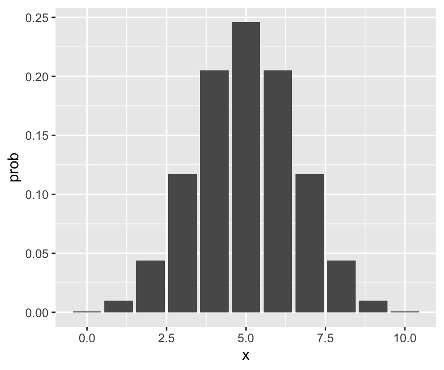
ggplot(data = dat_binom) +
  geom_col(aes(x = x, y = prob)) +
scale_x_continuous(breaks = 0:10) 
ggplot(data = dat_binom) +
  geom_col(aes(x = x, y = prob), width = .2) +
  scale_x_continuous(breaks = 0:10)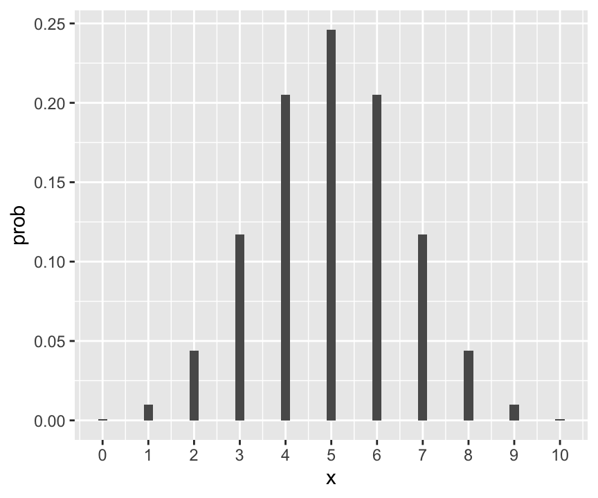
ggplot(data = dat_binom) +
  geom_col(aes(x = x, y = prob), width = .2) +
  scale_x_continuous(breaks = 0:10) +
  theme_minimal(base_size = 18)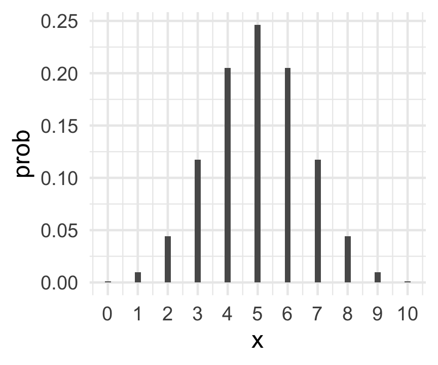
Binomial distribution: CDF
\[F(x) = P(X\leq x) = \sum_{y\leq x} P(X=y)\]
p1 <- ggplot(data = dat_binom) +
  geom_step(aes(x = x, y = cprob)) +
  scale_x_continuous(breaks = 0:10) +
  theme_bw(base_size = 18)
p1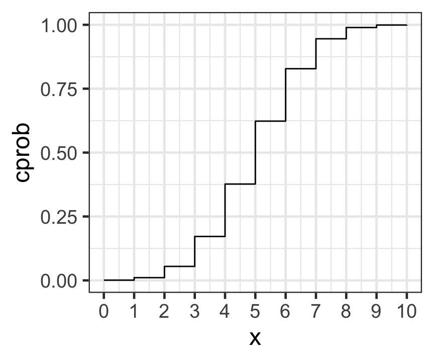
dat1 = tibble(x = dat_binom$x[-1],
              y = dat_binom$cprob[-11])
#
p1 +
  geom_point(aes(x = x, y = cprob), size = 4) +
  geom_point(data = dat1, aes(x = x, y = y),
shape=1, size = 3) 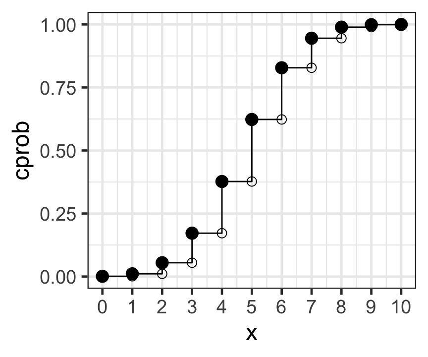
Normal distribution: PDF
ggplot(dat_norm) +
  geom_line(aes(x, f), size = 2) +
  theme_bw(base_size = 18)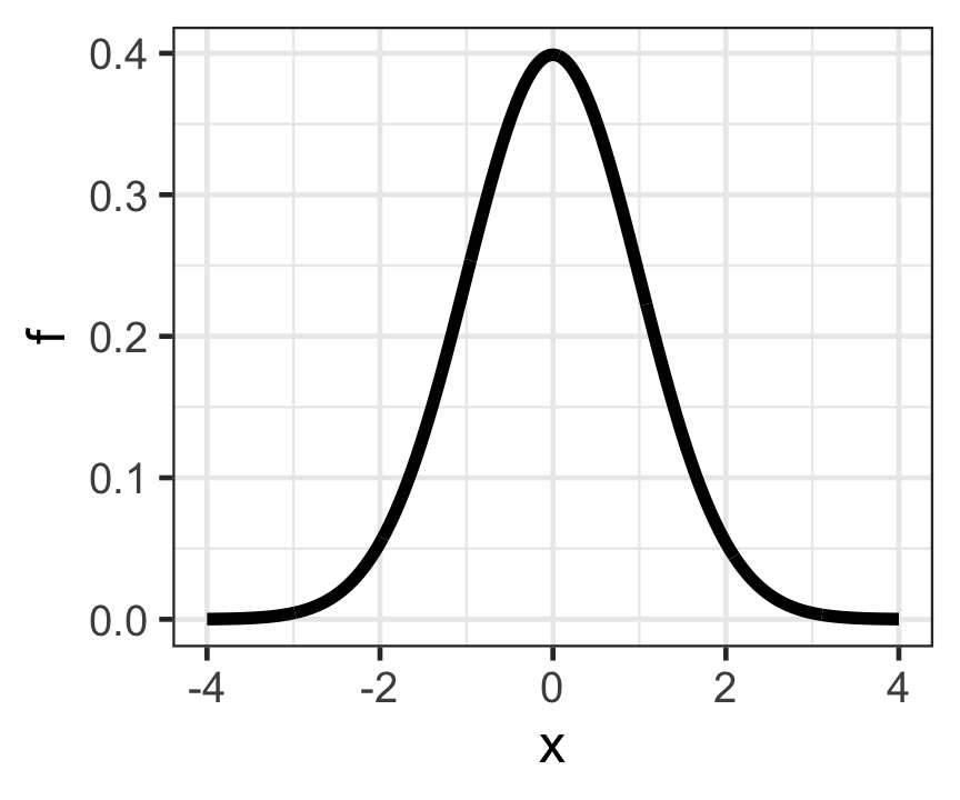
Normal distribution: CDF
ggplot(dat_norm) +
  geom_line(aes(x, F), size = 2) +
  theme_bw(base_size = 18)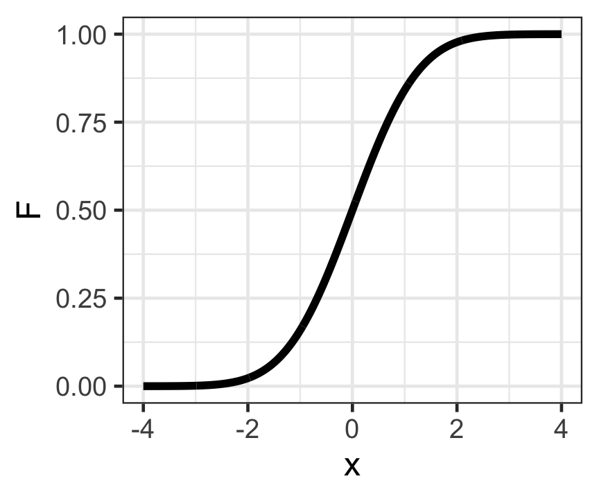
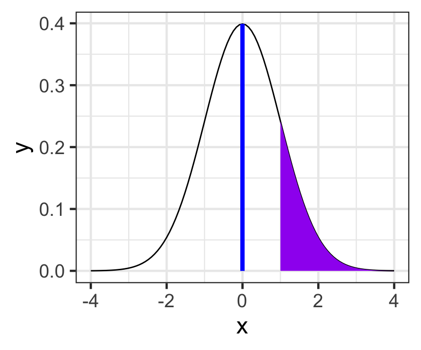
Standard normal distribution: PDF
ggplot(data = tibble(x = c(-4, 4))) +
  stat_function(
    mapping = aes(x = x), fun = dnorm,
    args = list(mean = 0, sd = 1), geom = "line") +
  theme_bw(base_size = 18)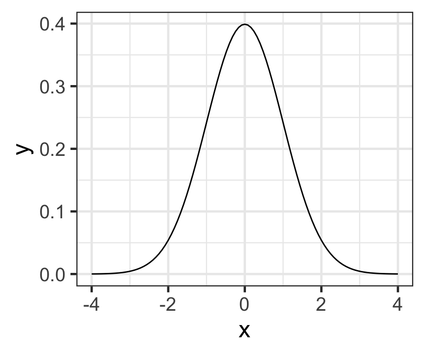
ggplot(data = tibble(x = c(-4, 4))) +
  stat_function(
    mapping = aes(x = x), fun = dnorm,
    geom = "line") +
  stat_function(
    mapping = aes(x = x), fun = dnorm,
    geom = "area", xlim = c(1, 4), fill = "purple") +
  theme_bw(base_size = 18)
- Unspecified
argsargument instat_function()corresponds to standard normal distribution
ggplot(data = tibble(x = c(-4, 4))) +
  stat_function(
    mapping = aes(x = x), fun = dnorm,
    geom = "line") +
  stat_function(
    mapping = aes(x = x), fun = dnorm,
    geom = "area", xlim = c(1, 4), fill = "purple") +
  geom_segment(
    aes(x = 0, xend = 0, y = 0, yend = dnorm(0)),
    col = "blue", size = 1.5) +
  theme_bw(base_size = 18)