1 Getting Started with R

Author

Affiliation

Md Rasel Biswas

IASDS, University of Dhaka

1 Getting Started with R

When you type something into the Console, R will give you a reply. For example:
```
2 + 4
#> [1] 6
```
As expected, R returned 6.

Note

You can ignore the [1] shown in the output for now. It indicates that the line begins with the first element of the result.

R can also be used as a calculator.

(59 + 73 + 2) / 3
#> [1] 44.66667
10^(3 + 1)
#> [1] 10000

Note

Arithmetic operators in R are similar to those used in most other computer applications.

2 Arithmetic Operators

Description	Operator
Addition	`+`
Subtraction	`-`
Multiplication	`*`
Division	`/`
Exponentiation	`^` or `**`
Integer division	`x %/% y` (e.g., `10 %/% 3` is `3`)
Modulus (remainder)	`x %% y` (e.g., `10 %% 3` is `1`)

3 Exercise 1.1

Use R to calculate the following:
- \(5^2\)
- Add 8 to 22 and then multiply the result by 3.
- Divide 8 by 2.5 and then divide the result by 3.

Notice

These calculations do not create objects that are remembered by R.

4 Creating Objects

To store calculations or values in R, we assign them to objects.
The assignment operators <- or = can be used, but <- is preferred because = also has other uses.
```
my_obj <- 48
```
Now that we have created this object, R will remember it during the current session.
All created objects are stored in the current workspace. In RStudio, you can see them under the Environment tab in the top-right pane.

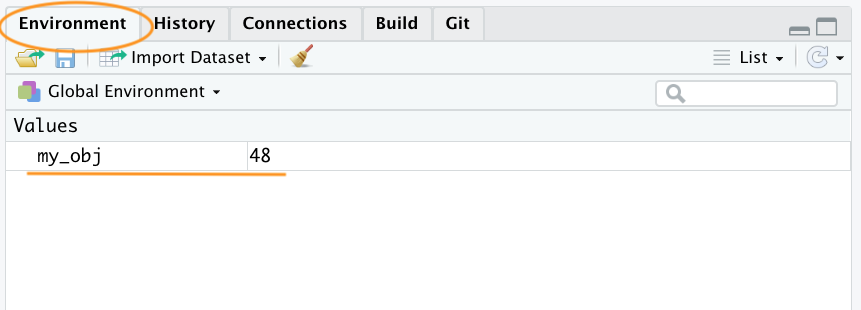
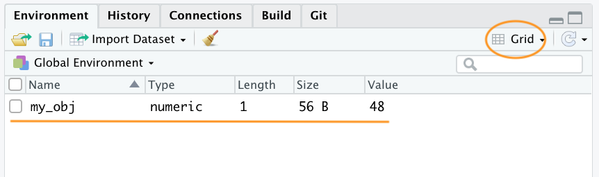
If you switch from List to Grid view in the Environment tab, RStudio will show:
- the type, such as numeric;
- the length, or number of values;
- the size in memory; and
- the stored value.

Objects can hold different types of values. For example:
```
my_obj2 <- "R is cool"
```
Here, we created my_obj2, which stores the character string "R is cool".

Note

Character strings must be enclosed in quotation marks.

If you forget the quotation marks, R will return an error.

my_obj2 <- R is cool
#> Error in parse(text = input): <text>:1:14: unexpected symbol
#> 1: my_obj2 <- R is
#>                  ^

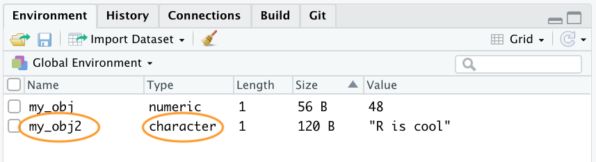
Our workspace now contains both my_obj and my_obj2.

To change the value of an existing object, reassign it:
```
my_obj2 <- 1024
```
Now my_obj2 holds a numeric value instead of a character string.

You can perform operations using objects. For example:
```
my_obj3 <- my_obj + my_obj2
my_obj3
#> [1] 1072
```
This creates my_obj3 with the value \(48 + 1024 = 1072\).

If you try to add two character strings:

char_obj <- "hello"
char_obj2 <- "world!"
char_obj3 <- char_obj + char_obj2
#> Error in `char_obj + char_obj2`:
#> ! non-numeric argument to binary operator

R will return an error because character strings cannot be added using +.

Another common error is object not found.

my_obj <- 48
my_obj4 <- my_obj + no_obj
#> Error:
#> ! object 'no_obj' not found

Here, no_obj has not been created, so the operation fails.

5 Naming Objects

In R, object names are case-sensitive. For example, my_obj and My_obj are different objects.
Valid object names can include:
- letters (a-z, A-Z);
- digits (0-9);
- a dot .; and
- an underscore _.
Rules:
- Names cannot start with a number or an underscore _.
- Names can start with a dot, but the dot cannot be followed by a number.
- Non-standard names must be enclosed in backticks.
Good practice: use meaningful names to make your code easier to read.
Avoid using the names of existing R functions or reserved words, such as mean, log, exp, TRUE, and c.

6 Exercise 1.2

Create an object x1 with the value 73.
Create x2 as the result of \(101 + 36\).
Multiply x1 and x2 and store the result in x3.
Subtract 1 from x3 and calculate its fourth root.
The answer should be 10.

7 Use of Brackets

Parentheses ( ) are used to group expressions and control the order of operations. They must be matched.
```
((3 + 12) / 3 + 8)
#> [1] 13
```
Curly braces { } are generally used to group several expressions, such as inside functions or loops.
```
{
  x <- 10 + 2
  x + 5
}
#> [1] 17
```
Square brackets [ ] are used for indexing or selecting elements, not for grouping arithmetic expressions.
```
[2 + 7] / 3
#> Error in parse(text = input): <text>:1:1: unexpected '['
#> 1: [
#>     ^
```

8 R Functions

Functions are pre-written pieces of code that perform specific tasks.
Some examples are given below.

Description	Function	Example
Square root	`sqrt`	`sqrt(225)`
Natural logarithm	`log`	`log(50)`
Exponential	`exp`	`exp(3)`
Absolute value	`abs`	`abs(-10)`
Factorial	`factorial`	`factorial(6)`
Sine function	`sin`	`sin(25)`
Inverse cosine	`acos`	`acos(-1)`

The general structure of a function is:

function_name(arg1 = val1, arg2 = val2, ...)

For example:
```
sqrt(25)
#> [1] 5
sqrt(x = 25)
#> [1] 5
```
Both return 5.

Note

Inputs to a function are called arguments and are placed inside parentheses ( ).
Multiple arguments are separated by commas.

9 Some Useful Built-in Functions

round(3.567, digits = 2)
#> [1] 3.57
floor(3.567)
#> [1] 3
ceiling(3.567)
#> [1] 4
pi   # Not a function, but a useful built-in value
#> [1] 3.141593

10 R Ignores Extra Spaces

(1 + 2)     ^     3
#> [1] 27
    ( 1 +  2)    ^ 3
#> [1] 27

You can add spaces freely between elements of an expression.

However, spaces inside a value or object name may cause errors.

3   .14
#> Error in parse(text = input): <text>:1:5: unexpected numeric constant
#> 1: 3   .14
#>         ^

11 Commenting Code

Use # to write comments. R ignores everything after # on that line.

# Calculating BMI
weight <- 70   # in kg
height <- 1.7  # in metres
bmi <- weight / height^2
bmi
#> [1] 24.22145

12 Running R Scripts

Instead of typing code line by line in the Console, you can save it in an R script, which has the extension .R.
In RStudio, you can run the current line or selected lines using Ctrl + Enter on Windows or Command + Enter on macOS.

12.1 From the R Console

source("my_script.R")

Note

Make sure the script file is saved in the current working directory.
If it is in another folder, provide the file path.
Example: source("C:/Users/Rasel/Documents/my_script.R")

12.2 From the Terminal

Rscript my_script.R

Tip

source() runs the script inside the current R session, so the created objects remain available.
Rscript runs the script in a fresh session, so the created objects do not remain in your current RStudio session.

13 Exercise 1.3

Why does the following code not work?

my_variable <- 10
my_varıable
#> Error:
#> ! object 'my_varıable' not found

14 Exercise 1.4

Create an object myObject with a value between 1 and 100.
Add 13 to myObject and update the object.
Check whether myObject is divisible by 2, 3, 13, or 21.
Find how many complete times 5 fits into myObject.

15 Exercise 1.5

Save the following code in a file named practice.R:
```
x <- 5
y <- 10
print(x + y)
```
Run it using source("practice.R") from the R Console.
Run it using Rscript practice.R from the Terminal.