3 Working with Vectors
1 Vectors
-
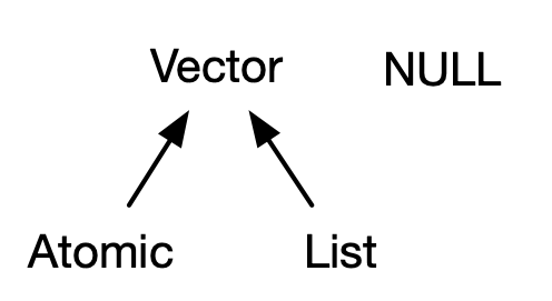
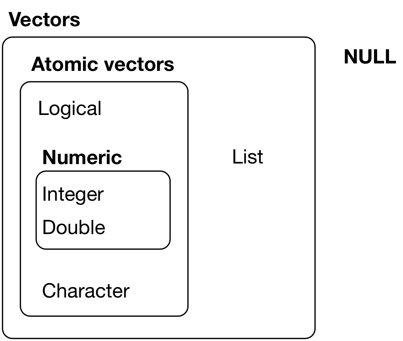
A variable or an R object with more than one value is known as a vector, and in R, there are two types of vectors: atomic vectors and lists
Atomic vector consists of the same type of elements, e.g. all doubles or all characters.
List can have elements of different data types, i.e. one element of a list could be a numeric value, and the other could be a character value. [More on lists later]
Most of the time, atomic vectors are just called vectors (we’ve already done this in the last section, and we’ll keep doing it throughout the course!).
While lists are also technically vectors, we like to keep things clear by simply calling them “lists.” It makes things easier to understand


2 Combining vectors
- The function
c()merges an arbitrary number of vectors to one vector
- R will quite happily do arithmetic operations with vectors as well
x+3
#> [1] 13 18
x/3
#> [1] 3.333333 5.000000
3 Arithmetic operations
- Functions work on vectors as they do on individual objects.
log(x)
#> [1] 2.302585 2.708050- Arithmetic operations can also be done with two vectors
4 The recycling rule of vectors
It is not necessary to have vectors of the same length in an expression
If two vectors in an expression are not of the same length then the shorter one will be repeated until it has the same length as the longer one.
5 Some vector functions
6 Summary statistics on vectors
| Function | Example | Output |
|---|---|---|
sum(), prod()
|
sum(1:10) |
55 |
min(), max()
|
min(1:10) |
1 |
mean(), median()
|
median(1:10) |
5.5 |
sd(), var()
|
sd(1:10) |
3.0276504 |
quantile() |
quantile(1:10) |
1, 3.25, 5.5, 7.75, 10 |
- Check the help pages of the R functions related to these summary statistics
7 Extracting elements of vectors:
- To extract (also known as indexing or subscripting) one or more values (more generally known as elements) from a vector, we use the square bracket
[ ]notation
7.1 Indexing vectors with [] (Positional indexing)
A vector of the age of five children
age <- c(11, 9, 8, 10, 5)
age
#> [1] 11  9  8 10  5
Age of a specific child, say the third child
age[3]
#> [1] 8The positional index starts at 1 rather than 0 like some other programming languages (e.g. C, Python)
7.2 Indexing vectors with [] (Logical indexing)
age
#> [1] 11  9  8 10  5
age >= 8
#> [1]  TRUE  TRUE  TRUE  TRUE FALSE
Number of children with age 8 years or more
sum(age >= 8)
#> [1] 4
Select the observations greater than 8 years
age[age >= 8]
#> [1] 11  9  8 10
age
#> [1] 11 9 8 10 5Children with age 11 or 8 years
Children with ages not equal to 11 or 8 years
age
#> [1] 11 9 8 10 5Observations with age greater than 9 or less than 8
age[age > 9 | age < 8]
#> [1] 11 10  5
Observations with ages between 8 to 10 inclusive
age[age >= 8 & age <= 10]
#> [1]  9  8 10
The mean age of observations between 8 to 10 inclusive
mean(age[age >= 8 & age <= 10])
#> [1] 9
8 Replacing elements
Changing values of a vector
age <- c(11, 9, 8, 10, 5)
age1 <- age
age1
#> [1] 11  9  8 10  5
age2 <- age
age2
#> [1] 11  9  8 10  5
Change the first child’s age to 15
age1[1] <- 15
age1
#> [1] 15  9  8 10  5
Change it to 20 if it is greater than 9
age2[age2 > 9] <- 20
age2
#> [1] 20  9  8 20  5
9 Ordering elements
10 Exercise 3
The following code generates a vector nage of size 1000.
-
Show that the number of observations
greater than 70 is 176
less than 40 is 185
equal to 39 is 19
greater than 77 or less than 35 is 140
between 50 and 55 (inclusive) is 110
What percentage of observations lies between 70 to 75 (inclusive)?
11 Missing values
In R, missing values are coded as
NAmeaning ‘Not available’Most of the R functions return missing value (i.e.
NA) if any input vector contains a missing value
- Most of the R functions have an argument
na.rm, which takes a logical value to include (or exclude) the missing value in (from) the calculation
mval
#> [1] 12 13 14 15 NA
mean(mval)
#> [1] NA12 Coercion
In R, atomic vectors are homogeneous, i.e., all elements of an atomic vector will be of the same data type
If you attempt to create an atomic vector with more than one data type, e.g.
nvec <- c(1, 2, "all"), then R will create an atomic vector, i.e. all elements ofnvecwill be of the same data type, which is known as coercion
nvec <- c(1, 2, "all")
nvec
#> [1] "1" "2" "all"typeof(nvec)
#> [1] "character"- In R, coercion occurs in the following (decreasing) order of precedence
- Character 2. Numeric 3. Integer 4. Logical
12.1 Explicit coercion
- Objects can be explicitly coerced from one type to another using
as.**functions, if available
x <- 0:5
typeof(x)
#> [1] "integer"
as.numeric(x)
#> [1] 0 1 2 3 4 5
as.logical(x)
#> [1] FALSE  TRUE  TRUE  TRUE  TRUE  TRUE
as.character(x)
#> [1] "0" "1" "2" "3" "4" "5"- Nonsensical coercion results in
NAs
x <- c("a", "b", "0", "522")
as.numeric(x)
#> [1]  NA  NA   0 522
as.logical(x)
#> [1] NA NA NA NA
13 Attributes
An attribute is a piece of information that you can attach to an atomic vector (or any R object) and it won’t affect any of the values in the object, and it will usually not appear when displaying the object.
Attributes are metadata and R will normally ignore it, but some R functions will check for specific attributes
Atomic vectors can be transformed into some other important R data structures, e.g., matrices, arrays, factors, or date-times by adding attributes
Attributes can be retrieved and modified by
attr()orattributes()
# an atomic vector that initially has no attributes
die <- 1:6
attributes(die)
#> NULL
# Setting an attribute named "x"
attr(die, "x") <- "abcd"
attributes(die)
#> $x
#> [1] "abcd"
# Now it has an attribute
die
#> [1] 1 2 3 4 5 6
#> attr(,"x")
#> [1] "abcd"Two mostly used attributes are:
- names, a character vector giving each element a name.
- dim, short for dimensions, an integer vector, used to turn vectors into matrices or arrays.
13.1 Names
names is one of the common attributes of an R object. We can set names to an atomic vector in various ways. Two of them are:
# Subsetting vector by names
x[["a"]]
#> [1] 113.2 Dimensions
- An atomic vector can be transformed into \(n\)-dimensional array by adding a dimension attribute with
dim
# Modifying the dim attribute
dim(die1) <- c(3, 2)
die1
#>      [,1] [,2]
#> [1,]    1    4
#> [2,]    2    5
#> [3,]    3    6
# See the attributes
attributes(die1)
#> $dim
#> [1] 3 2R will always use the first value in
dimfor the number of rows and the second value for the number of columnsR always fills up each matrix by columns, instead of by rows
R functions
matrix()andarray()can be used to control how the columns and rows of a matrix will be arranged (More on next section)