11 Data Transformation

Author

Affiliation

Md Rasel Biswas

ISRT, University of Dhaka

1 Tibble review

tibble() is similar to data.frame(), but has some advantages
A data frame can be transformed into a tibble() by as_tibble()
E.g. create a tibble object mtcars_t from a data frame mtcars

mtcars_t <- as_tibble(mtcars)
mtcars_t
#> # A tibble: 32 × 11
#>      mpg   cyl  disp    hp  drat    wt  qsec    vs    am  gear  carb
#>    <dbl> <dbl> <dbl> <dbl> <dbl> <dbl> <dbl> <dbl> <dbl> <dbl> <dbl>
#>  1  21       6  160    110  3.9   2.62  16.5     0     1     4     4
#>  2  21       6  160    110  3.9   2.88  17.0     0     1     4     4
#>  3  22.8     4  108     93  3.85  2.32  18.6     1     1     4     1
#>  4  21.4     6  258    110  3.08  3.22  19.4     1     0     3     1
#>  5  18.7     8  360    175  3.15  3.44  17.0     0     0     3     2
#>  6  18.1     6  225    105  2.76  3.46  20.2     1     0     3     1
#>  7  14.3     8  360    245  3.21  3.57  15.8     0     0     3     4
#>  8  24.4     4  147.    62  3.69  3.19  20       1     0     4     2
#>  9  22.8     4  141.    95  3.92  3.15  22.9     1     0     4     2
#> 10  19.2     6  168.   123  3.92  3.44  18.3     1     0     4     4
#> # ℹ 22 more rows

2 Penguins data

The palmerpenguins::penguins data contains size measurements for three penguin species observed on three islands in the Palmer Archipelago, Antarctica.

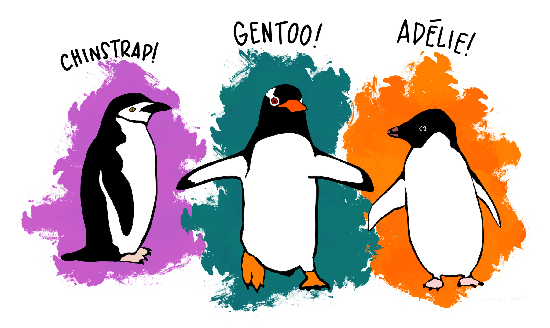
These data were collected from 2007 - 2009 by Dr. Kristen Gorman

The penguins data contains information (8 variables) on 344 penguins
Load the package palmerpenguins to access the penguins data

library(palmerpenguins)
data(penguins)
glimpse(penguins)
#> Rows: 344
#> Columns: 8
#> $ species           <fct> Adelie, Adelie, Adelie, Adelie, Adelie, Adelie, Adel…
#> $ island            <fct> Torgersen, Torgersen, Torgersen, Torgersen, Torgerse…
#> $ bill_length_mm    <dbl> 39.1, 39.5, 40.3, NA, 36.7, 39.3, 38.9, 39.2, 34.1, …
#> $ bill_depth_mm     <dbl> 18.7, 17.4, 18.0, NA, 19.3, 20.6, 17.8, 19.6, 18.1, …
#> $ flipper_length_mm <int> 181, 186, 195, NA, 193, 190, 181, 195, 193, 190, 186…
#> $ body_mass_g       <int> 3750, 3800, 3250, NA, 3450, 3650, 3625, 4675, 3475, …
#> $ sex               <fct> male, female, female, NA, female, male, female, male…
#> $ year              <int> 2007, 2007, 2007, 2007, 2007, 2007, 2007, 2007, 2007…

3 Overview of `dplyr`

dplyr: A powerful package for data manipulation with a consistent and flexible grammar.
dplyr package is helpful for different types of data transformations (e.g. creating new variables, computing summaries, renaming variables, reorders the observations, etc).
dplyr has versatile verbs to handle most data manipulation tasks.
It has a unified syntax:
- first argument is a data frame
- output is always a data frame

dplyr’s verbs are organized into four groups based on what they operate on:
- rows,
- columns,
- groups,
- tables

4 Verbs for Rows

Two most important verbs that operate on rows without changing the columns:

filter() keeps rows based on the values of the columns (variables)
arrange() reorders the rows (observations)
distinct() which finds rows with unique values.
- but it can also optionally modify the columns

4.1 `filter()`

Filter rows with `filter()`

The function filter() allows to obtain a subset of observations based on given conditions
- For example, we could find all the penguins of Chinstrap species

filter(penguins, species == "Chinstrap")

Equivalently,

penguins |> 
  filter(species == "Chinstrap") 
#> # A tibble: 68 × 8
#>    species   island bill_length_mm bill_depth_mm flipper_length_mm body_mass_g
#>    <fct>     <fct>           <dbl>         <dbl>             <int>       <int>
#>  1 Chinstrap Dream            46.5          17.9               192        3500
#>  2 Chinstrap Dream            50            19.5               196        3900
#>  3 Chinstrap Dream            51.3          19.2               193        3650
#>  4 Chinstrap Dream            45.4          18.7               188        3525
#>  5 Chinstrap Dream            52.7          19.8               197        3725
#>  6 Chinstrap Dream            45.2          17.8               198        3950
#>  7 Chinstrap Dream            46.1          18.2               178        3250
#>  8 Chinstrap Dream            51.3          18.2               197        3750
#>  9 Chinstrap Dream            46            18.9               195        4150
#> 10 Chinstrap Dream            51.3          19.9               198        3700
#> # ℹ 58 more rows
#> # ℹ 2 more variables: sex <fct>, year <int>

We can use >, >=, <, <=, ==, and != to write conditions
We can combine multiple conditions with
- & or , \(\rightarrow\) “and”
- | \(\rightarrow\) “or”

Question: Find Chinstrap penguins whose bill length is greater than 52 mm

penguins |>
  filter(species == "Chinstrap", bill_length_mm > 52)
#> # A tibble: 7 × 8
#>   species   island bill_length_mm bill_depth_mm flipper_length_mm body_mass_g
#>   <fct>     <fct>           <dbl>         <dbl>             <int>       <int>
#> 1 Chinstrap Dream            52.7          19.8               197        3725
#> 2 Chinstrap Dream            58            17.8               181        3700
#> 3 Chinstrap Dream            52.8          20                 205        4550
#> 4 Chinstrap Dream            54.2          20.8               201        4300
#> 5 Chinstrap Dream            53.5          19.9               205        4500
#> 6 Chinstrap Dream            52.2          18.8               197        3450
#> 7 Chinstrap Dream            55.8          19.8               207        4000
#> # ℹ 2 more variables: sex <fct>, year <int>

Question: Find the penguins of the types Chinstrap or Gentoo

penguins |>
  filter(species == "Chinstrap" | species == "Gentoo") 
#> # A tibble: 192 × 8
#>    species island bill_length_mm bill_depth_mm flipper_length_mm body_mass_g
#>    <fct>   <fct>           <dbl>         <dbl>             <int>       <int>
#>  1 Gentoo  Biscoe           46.1          13.2               211        4500
#>  2 Gentoo  Biscoe           50            16.3               230        5700
#>  3 Gentoo  Biscoe           48.7          14.1               210        4450
#>  4 Gentoo  Biscoe           50            15.2               218        5700
#>  5 Gentoo  Biscoe           47.6          14.5               215        5400
#>  6 Gentoo  Biscoe           46.5          13.5               210        4550
#>  7 Gentoo  Biscoe           45.4          14.6               211        4800
#>  8 Gentoo  Biscoe           46.7          15.3               219        5200
#>  9 Gentoo  Biscoe           43.3          13.4               209        4400
#> 10 Gentoo  Biscoe           46.8          15.4               215        5150
#> # ℹ 182 more rows
#> # ℹ 2 more variables: sex <fct>, year <int>

There’s a useful shortcut when you’re combining | and ==. That is: %in%

penguins |>
  filter(species %in% c("Chinstrap", "Gentoo")) 
#> # A tibble: 192 × 8
#>    species island bill_length_mm bill_depth_mm flipper_length_mm body_mass_g
#>    <fct>   <fct>           <dbl>         <dbl>             <int>       <int>
#>  1 Gentoo  Biscoe           46.1          13.2               211        4500
#>  2 Gentoo  Biscoe           50            16.3               230        5700
#>  3 Gentoo  Biscoe           48.7          14.1               210        4450
#>  4 Gentoo  Biscoe           50            15.2               218        5700
#>  5 Gentoo  Biscoe           47.6          14.5               215        5400
#>  6 Gentoo  Biscoe           46.5          13.5               210        4550
#>  7 Gentoo  Biscoe           45.4          14.6               211        4800
#>  8 Gentoo  Biscoe           46.7          15.3               219        5200
#>  9 Gentoo  Biscoe           43.3          13.4               209        4400
#> 10 Gentoo  Biscoe           46.8          15.4               215        5150
#> # ℹ 182 more rows
#> # ℹ 2 more variables: sex <fct>, year <int>

Exercise 1

Create a subset from penguins that only contains Gentoo penguins with a bill depth greater than or equal to 15.5 millimeters.
Create a subset from penguins that contains observations for male penguins recorded at Dream or Biscoe Islands.
Create a subset from penguins that contains penguins that are either Gentoo or have a body mass greater than 4500 g.

4.2 `arrange()`

Arrange rows with `arrange()`

arrange() reorders the observations by one or more variables (column names)
As inputs, arrange() takes a data frame and a set of column names (variables) to order by
If more than one columns are used in the arguments then each additional column will be used to break ties in the values of preceding column
Default is ascending order (lowest to highest)

penguins |> 
  arrange(bill_length_mm)
#> # A tibble: 344 × 8
#>    species island    bill_length_mm bill_depth_mm flipper_length_mm body_mass_g
#>    <fct>   <fct>              <dbl>         <dbl>             <int>       <int>
#>  1 Adelie  Dream               32.1          15.5               188        3050
#>  2 Adelie  Dream               33.1          16.1               178        2900
#>  3 Adelie  Torgersen           33.5          19                 190        3600
#>  4 Adelie  Dream               34            17.1               185        3400
#>  5 Adelie  Torgersen           34.1          18.1               193        3475
#>  6 Adelie  Torgersen           34.4          18.4               184        3325
#>  7 Adelie  Biscoe              34.5          18.1               187        2900
#>  8 Adelie  Torgersen           34.6          21.1               198        4400
#>  9 Adelie  Torgersen           34.6          17.2               189        3200
#> 10 Adelie  Biscoe              35            17.9               190        3450
#> # ℹ 334 more rows
#> # ℹ 2 more variables: sex <fct>, year <int>

# arrange in descending order
penguins |>
  arrange(desc(bill_depth_mm))
#> # A tibble: 344 × 8
#>    species   island   bill_length_mm bill_depth_mm flipper_length_mm body_mass_g
#>    <fct>     <fct>             <dbl>         <dbl>             <int>       <int>
#>  1 Adelie    Torgers…           46            21.5               194        4200
#>  2 Adelie    Torgers…           38.6          21.2               191        3800
#>  3 Adelie    Dream              42.3          21.2               191        4150
#>  4 Adelie    Torgers…           34.6          21.1               198        4400
#>  5 Adelie    Dream              39.2          21.1               196        4150
#>  6 Adelie    Biscoe             41.3          21.1               195        4400
#>  7 Chinstrap Dream              54.2          20.8               201        4300
#>  8 Adelie    Torgers…           42.5          20.7               197        4500
#>  9 Adelie    Biscoe             39.6          20.7               191        3900
#> 10 Chinstrap Dream              52            20.7               210        4800
#> # ℹ 334 more rows
#> # ℹ 2 more variables: sex <fct>, year <int>

# arrange with more than one variables
penguins |> 
  arrange(desc(bill_depth_mm), 
          desc(flipper_length_mm))
#> # A tibble: 344 × 8
#>    species   island   bill_length_mm bill_depth_mm flipper_length_mm body_mass_g
#>    <fct>     <fct>             <dbl>         <dbl>             <int>       <int>
#>  1 Adelie    Torgers…           46            21.5               194        4200
#>  2 Adelie    Torgers…           38.6          21.2               191        3800
#>  3 Adelie    Dream              42.3          21.2               191        4150
#>  4 Adelie    Torgers…           34.6          21.1               198        4400
#>  5 Adelie    Dream              39.2          21.1               196        4150
#>  6 Adelie    Biscoe             41.3          21.1               195        4400
#>  7 Chinstrap Dream              54.2          20.8               201        4300
#>  8 Chinstrap Dream              52            20.7               210        4800
#>  9 Adelie    Torgers…           42.5          20.7               197        4500
#> 10 Adelie    Biscoe             39.6          20.7               191        3900
#> # ℹ 334 more rows
#> # ℹ 2 more variables: sex <fct>, year <int>

4.3 `distinct()`

Find unique rows with `distinct()`

distinct() finds all the unique rows in a dataset

# Remove duplicate rows, if any
penguins |>
  distinct()
#> # A tibble: 344 × 8
#>    species island    bill_length_mm bill_depth_mm flipper_length_mm body_mass_g
#>    <fct>   <fct>              <dbl>         <dbl>             <int>       <int>
#>  1 Adelie  Torgersen           39.1          18.7               181        3750
#>  2 Adelie  Torgersen           39.5          17.4               186        3800
#>  3 Adelie  Torgersen           40.3          18                 195        3250
#>  4 Adelie  Torgersen           NA            NA                  NA          NA
#>  5 Adelie  Torgersen           36.7          19.3               193        3450
#>  6 Adelie  Torgersen           39.3          20.6               190        3650
#>  7 Adelie  Torgersen           38.9          17.8               181        3625
#>  8 Adelie  Torgersen           39.2          19.6               195        4675
#>  9 Adelie  Torgersen           34.1          18.1               193        3475
#> 10 Adelie  Torgersen           42            20.2               190        4250
#> # ℹ 334 more rows
#> # ℹ 2 more variables: sex <fct>, year <int>

Most of the time, however, you’ll want the distinct combination of some variables, so you can also optionally supply column names

#Find all unique species and year pairs
penguins |>
  distinct(species, year)
#> # A tibble: 9 × 2
#>   species    year
#>   <fct>     <int>
#> 1 Adelie     2007
#> 2 Adelie     2008
#> 3 Adelie     2009
#> 4 Gentoo     2007
#> 5 Gentoo     2008
#> 6 Gentoo     2009
#> 7 Chinstrap  2007
#> 8 Chinstrap  2008
#> 9 Chinstrap  2009

If you want to find the number of occurrences instead, you’re better off swapping distinct() for count().
- With the sort = TRUE argument, you can arrange them in descending order of the number of occurrences

#Find count for species and year pairs
penguins |>
  count(species, year, sort = TRUE)
#> # A tibble: 9 × 3
#>   species    year     n
#>   <fct>     <int> <int>
#> 1 Adelie     2009    52
#> 2 Adelie     2007    50
#> 3 Adelie     2008    50
#> 4 Gentoo     2008    46
#> 5 Gentoo     2009    44
#> 6 Gentoo     2007    34
#> 7 Chinstrap  2007    26
#> 8 Chinstrap  2009    24
#> 9 Chinstrap  2008    18

5 Verbs for Columns

There are four important verbs that affect the columns without changing the rows:

mutate() creates new columns that are derived from the existing columns,
select() changes which columns are present, and
rename() changes the names of the columns

5.1 `mutate()`

Add new variables with `mutate()`

mutate() is used to create new variables to the existing data frame
E.g. create a new variable body_mass_kg (body mass in kg) by body_mass_g/1000

penguins |>
  mutate(body_mass_kg = body_mass_g / 1000)
#> # A tibble: 344 × 9
#>    species island    bill_length_mm bill_depth_mm flipper_length_mm body_mass_g
#>    <fct>   <fct>              <dbl>         <dbl>             <int>       <int>
#>  1 Adelie  Torgersen           39.1          18.7               181        3750
#>  2 Adelie  Torgersen           39.5          17.4               186        3800
#>  3 Adelie  Torgersen           40.3          18                 195        3250
#>  4 Adelie  Torgersen           NA            NA                  NA          NA
#>  5 Adelie  Torgersen           36.7          19.3               193        3450
#>  6 Adelie  Torgersen           39.3          20.6               190        3650
#>  7 Adelie  Torgersen           38.9          17.8               181        3625
#>  8 Adelie  Torgersen           39.2          19.6               195        4675
#>  9 Adelie  Torgersen           34.1          18.1               193        3475
#> 10 Adelie  Torgersen           42            20.2               190        4250
#> # ℹ 334 more rows
#> # ℹ 3 more variables: sex <fct>, year <int>, body_mass_kg <dbl>

By default, mutate() adds new columns on the right side of your data

We can use the .before argument to add the variables to the left-hand side (.before=1 means before the 1st variable).

 penguins |> 
  mutate(body_mass_kg = body_mass_g / 1000,
         .before = 1)
#> # A tibble: 344 × 9
#>    body_mass_kg species island    bill_length_mm bill_depth_mm flipper_length_mm
#>           <dbl> <fct>   <fct>              <dbl>         <dbl>             <int>
#>  1         3.75 Adelie  Torgersen           39.1          18.7               181
#>  2         3.8  Adelie  Torgersen           39.5          17.4               186
#>  3         3.25 Adelie  Torgersen           40.3          18                 195
#>  4        NA    Adelie  Torgersen           NA            NA                  NA
#>  5         3.45 Adelie  Torgersen           36.7          19.3               193
#>  6         3.65 Adelie  Torgersen           39.3          20.6               190
#>  7         3.62 Adelie  Torgersen           38.9          17.8               181
#>  8         4.68 Adelie  Torgersen           39.2          19.6               195
#>  9         3.48 Adelie  Torgersen           34.1          18.1               193
#> 10         4.25 Adelie  Torgersen           42            20.2               190
#> # ℹ 334 more rows
#> # ℹ 3 more variables: body_mass_g <int>, sex <fct>, year <int>

Re-coding with `mutate()`

Suppose we want to classify penguins by their flipper size, so create a new variable flip_size, which will be either “large” or “short”
- “large” if flipper size is greater than 210 mm
- “short” if flipper size is less than or equal to 210 mm
if_else(condition, true, false) is used to obtain a variable with two levels depending on whether condition is satisfied or not

penguins |>
  mutate(
    flip_size = if_else(
      flipper_length_mm > 210, "large", "short")
    )
#> # A tibble: 344 × 9
#>    species island    bill_length_mm bill_depth_mm flipper_length_mm body_mass_g
#>    <fct>   <fct>              <dbl>         <dbl>             <int>       <int>
#>  1 Adelie  Torgersen           39.1          18.7               181        3750
#>  2 Adelie  Torgersen           39.5          17.4               186        3800
#>  3 Adelie  Torgersen           40.3          18                 195        3250
#>  4 Adelie  Torgersen           NA            NA                  NA          NA
#>  5 Adelie  Torgersen           36.7          19.3               193        3450
#>  6 Adelie  Torgersen           39.3          20.6               190        3650
#>  7 Adelie  Torgersen           38.9          17.8               181        3625
#>  8 Adelie  Torgersen           39.2          19.6               195        4675
#>  9 Adelie  Torgersen           34.1          18.1               193        3475
#> 10 Adelie  Torgersen           42            20.2               190        4250
#> # ℹ 334 more rows
#> # ℹ 3 more variables: sex <fct>, year <int>, flip_size <chr>

To re-code a variable in more than two categories, case_when() function is used
For example, we are interested in classifying penguins into three categories (large, medium, and small) by their body mass where
- “small” (<=3000], “medium” (3000-4500), “large” (>=4500),

penguins |>
  mutate(
    mass_c = case_when(
      body_mass_g > 4500 ~ "large",
      body_mass_g > 3000 & 
        body_mass_g <= 4500 ~ "medium",
      body_mass_g <= 3000 ~ "small"
    ), .before = 1
  )
#> # A tibble: 344 × 9
#>    mass_c species island    bill_length_mm bill_depth_mm flipper_length_mm
#>    <chr>  <fct>   <fct>              <dbl>         <dbl>             <int>
#>  1 medium Adelie  Torgersen           39.1          18.7               181
#>  2 medium Adelie  Torgersen           39.5          17.4               186
#>  3 medium Adelie  Torgersen           40.3          18                 195
#>  4 <NA>   Adelie  Torgersen           NA            NA                  NA
#>  5 medium Adelie  Torgersen           36.7          19.3               193
#>  6 medium Adelie  Torgersen           39.3          20.6               190
#>  7 medium Adelie  Torgersen           38.9          17.8               181
#>  8 large  Adelie  Torgersen           39.2          19.6               195
#>  9 medium Adelie  Torgersen           34.1          18.1               193
#> 10 medium Adelie  Torgersen           42            20.2               190
#> # ℹ 334 more rows
#> # ℹ 3 more variables: body_mass_g <int>, sex <fct>, year <int>

5.2 `select()`

Select columns with `select()`

In practice, only a subset of variables from the original data frame are used, the original data frame may contain thousands of variables
select() is used to create a new data frame with the variables mentioned in the arguments (selected variables)
As inputs, a data frame, and column names to be selected are used in select()

Create a data frame with three variables:
- year, island, and species

penguins |>
  select(year, island, species)
#> # A tibble: 344 × 3
#>     year island    species
#>    <int> <fct>     <fct>  
#>  1  2007 Torgersen Adelie 
#>  2  2007 Torgersen Adelie 
#>  3  2007 Torgersen Adelie 
#>  4  2007 Torgersen Adelie 
#>  5  2007 Torgersen Adelie 
#>  6  2007 Torgersen Adelie 
#>  7  2007 Torgersen Adelie 
#>  8  2007 Torgersen Adelie 
#>  9  2007 Torgersen Adelie 
#> 10  2007 Torgersen Adelie 
#> # ℹ 334 more rows

names(penguins) 
#> [1] "species"           "island"            "bill_length_mm"   
#> [4] "bill_depth_mm"     "flipper_length_mm" "body_mass_g"      
#> [7] "sex"               "year"

A colon (:) can be used to select a number of consecutive variables

penguins |>
  select(species:body_mass_g) 
#> # A tibble: 344 × 6
#>    species island    bill_length_mm bill_depth_mm flipper_length_mm body_mass_g
#>    <fct>   <fct>              <dbl>         <dbl>             <int>       <int>
#>  1 Adelie  Torgersen           39.1          18.7               181        3750
#>  2 Adelie  Torgersen           39.5          17.4               186        3800
#>  3 Adelie  Torgersen           40.3          18                 195        3250
#>  4 Adelie  Torgersen           NA            NA                  NA          NA
#>  5 Adelie  Torgersen           36.7          19.3               193        3450
#>  6 Adelie  Torgersen           39.3          20.6               190        3650
#>  7 Adelie  Torgersen           38.9          17.8               181        3625
#>  8 Adelie  Torgersen           39.2          19.6               195        4675
#>  9 Adelie  Torgersen           34.1          18.1               193        3475
#> 10 Adelie  Torgersen           42            20.2               190        4250
#> # ℹ 334 more rows

We can also omit variables using the negative sign.

penguins |>
  select(species:bill_depth_mm, -island) 
#> # A tibble: 344 × 3
#>    species bill_length_mm bill_depth_mm
#>    <fct>            <dbl>         <dbl>
#>  1 Adelie            39.1          18.7
#>  2 Adelie            39.5          17.4
#>  3 Adelie            40.3          18  
#>  4 Adelie            NA            NA  
#>  5 Adelie            36.7          19.3
#>  6 Adelie            39.3          20.6
#>  7 Adelie            38.9          17.8
#>  8 Adelie            39.2          19.6
#>  9 Adelie            34.1          18.1
#> 10 Adelie            42            20.2
#> # ℹ 334 more rows

select() can also be used to rename a variable and reordering the sequence of variables

penguins |>
  select(species, year, bill_len = bill_length_mm) 
#> # A tibble: 344 × 3
#>    species  year bill_len
#>    <fct>   <int>    <dbl>
#>  1 Adelie   2007     39.1
#>  2 Adelie   2007     39.5
#>  3 Adelie   2007     40.3
#>  4 Adelie   2007     NA  
#>  5 Adelie   2007     36.7
#>  6 Adelie   2007     39.3
#>  7 Adelie   2007     38.9
#>  8 Adelie   2007     39.2
#>  9 Adelie   2007     34.1
#> 10 Adelie   2007     42  
#> # ℹ 334 more rows

select() has some helper functions that can be used to select a subset of variables
- starts_with("abc"), ends_with("th"), contains("co"), etc.

names(penguins) 
#> [1] "species"           "island"            "bill_length_mm"   
#> [4] "bill_depth_mm"     "flipper_length_mm" "body_mass_g"      
#> [7] "sex"               "year"

penguins |>
  select(starts_with("bill")) 
#> # A tibble: 344 × 2
#>    bill_length_mm bill_depth_mm
#>             <dbl>         <dbl>
#>  1           39.1          18.7
#>  2           39.5          17.4
#>  3           40.3          18  
#>  4           NA            NA  
#>  5           36.7          19.3
#>  6           39.3          20.6
#>  7           38.9          17.8
#>  8           39.2          19.6
#>  9           34.1          18.1
#> 10           42            20.2
#> # ℹ 334 more rows

5.3 `rename()`

If you want to keep all the existing variables and just want to rename a few, you can use rename() instead of select()

penguins |>
  rename(location = island)
#> # A tibble: 344 × 8
#>    species location  bill_length_mm bill_depth_mm flipper_length_mm body_mass_g
#>    <fct>   <fct>              <dbl>         <dbl>             <int>       <int>
#>  1 Adelie  Torgersen           39.1          18.7               181        3750
#>  2 Adelie  Torgersen           39.5          17.4               186        3800
#>  3 Adelie  Torgersen           40.3          18                 195        3250
#>  4 Adelie  Torgersen           NA            NA                  NA          NA
#>  5 Adelie  Torgersen           36.7          19.3               193        3450
#>  6 Adelie  Torgersen           39.3          20.6               190        3650
#>  7 Adelie  Torgersen           38.9          17.8               181        3625
#>  8 Adelie  Torgersen           39.2          19.6               195        4675
#>  9 Adelie  Torgersen           34.1          18.1               193        3475
#> 10 Adelie  Torgersen           42            20.2               190        4250
#> # ℹ 334 more rows
#> # ℹ 2 more variables: sex <fct>, year <int>

Practice 2

Starting with the penguins data, only keep the body_mass_g variable.
Starting with the penguins data, keep columns from bill_length_mm to body_mass_g, and year
Starting with the penguins data, keep all columns except island
From penguins, keep the species column and any columns that end with “mm”.

6 The pipe

We’ve shown you simple examples of the pipe above, but its real power arises when you start to combine multiple verbs.
E.g. We want to find the female Adelie penguins with the largest bill sizes.

penguins |>
  filter(species == "Adelie" & sex == "female") |>
  arrange(desc(bill_length_mm))
#> # A tibble: 73 × 8
#>    species island    bill_length_mm bill_depth_mm flipper_length_mm body_mass_g
#>    <fct>   <fct>              <dbl>         <dbl>             <int>       <int>
#>  1 Adelie  Dream               42.2          18.5               180        3550
#>  2 Adelie  Torgersen           41.1          17.6               182        3200
#>  3 Adelie  Torgersen           40.9          16.8               191        3700
#>  4 Adelie  Biscoe              40.5          17.9               187        3200
#>  5 Adelie  Torgersen           40.3          18                 195        3250
#>  6 Adelie  Torgersen           40.2          17                 176        3450
#>  7 Adelie  Dream               40.2          17.1               193        3400
#>  8 Adelie  Biscoe              39.7          17.7               193        3200
#>  9 Adelie  Biscoe              39.6          17.7               186        3500
#> 10 Adelie  Torgersen           39.6          17.2               196        3550
#> # ℹ 63 more rows
#> # ℹ 2 more variables: sex <fct>, year <int>

What would happen if we didn’t have the pipe?

We could nest each function call inside the previous call?

arrange(
  filter(
    penguins,
    species == "Adelie" & sex == "female"
    ),
  desc(bill_length_mm))

Or we could use a bunch of intermediate objects:

penguins1 <- filter(species == "Adelie" & sex == "female")
arrange(penguins1, desc(bill_length_mm))

While both forms do the work, the pipe generally produces data analysis code that is easier to write and read

Behind the scenes
x |> f(y) \(\rightarrow\) f(x, y)
x |> f(y) |> g(z) \(\rightarrow\) f(x, y) |> g(z) \(\rightarrow\) g(f(x, y), z)

6.1 Another pipe

There is another pipe operator (%>%) provided by the magrittr package
The magrittr package is included in the core tidyverse, so you can use %>% whenever you load the tidyverse
For simple cases, |> and %>% behave identically

penguins %>% 
  filter(species == "Adelie" & sex == "female") %>% 
  arrange(desc(bill_length_mm))
#> # A tibble: 73 × 8
#>    species island    bill_length_mm bill_depth_mm flipper_length_mm body_mass_g
#>    <fct>   <fct>              <dbl>         <dbl>             <int>       <int>
#>  1 Adelie  Dream               42.2          18.5               180        3550
#>  2 Adelie  Torgersen           41.1          17.6               182        3200
#>  3 Adelie  Torgersen           40.9          16.8               191        3700
#>  4 Adelie  Biscoe              40.5          17.9               187        3200
#>  5 Adelie  Torgersen           40.3          18                 195        3250
#>  6 Adelie  Torgersen           40.2          17                 176        3450
#>  7 Adelie  Dream               40.2          17.1               193        3400
#>  8 Adelie  Biscoe              39.7          17.7               193        3200
#>  9 Adelie  Biscoe              39.6          17.7               186        3500
#> 10 Adelie  Torgersen           39.6          17.2               196        3550
#> # ℹ 63 more rows
#> # ℹ 2 more variables: sex <fct>, year <int>

7 Exercise

In a piped sequence, starting from penguins:

Only keep observations for female penguins observed on Dream Island, then
Keep variables species and any variable starting with “bill”

Add a column to penguins that contains a new column flipper_m, which is the flipper_length_mm (flipper length in millimeters) converted to units of meters.

The year column in penguins is currently an integer. Add a new column named year_fct that is the year converted to a factor (hint: as.factor())
Starting with penguins, do the following within a single mutate() function:

Convert the species variable to a character
Add a new column (called flipper_cm with flipper length in centimeters)
Convert the island column to lowercase

8 Verbs for Groups

So far you’ve learned about functions that work with rows and columns.
dplyr gets even more powerful when you add in the ability to work with groups.
In this section, we’ll focus on the most important functions: group_by(), and summarise()

8.1 `group_by()`

Use group_by() to divide dataset into groups meaningful for your analysis

penguins |>
  group_by(species)
#> # A tibble: 344 × 8
#> # Groups:   species [3]
#>    species island    bill_length_mm bill_depth_mm flipper_length_mm body_mass_g
#>    <fct>   <fct>              <dbl>         <dbl>             <int>       <int>
#>  1 Adelie  Torgersen           39.1          18.7               181        3750
#>  2 Adelie  Torgersen           39.5          17.4               186        3800
#>  3 Adelie  Torgersen           40.3          18                 195        3250
#>  4 Adelie  Torgersen           NA            NA                  NA          NA
#>  5 Adelie  Torgersen           36.7          19.3               193        3450
#>  6 Adelie  Torgersen           39.3          20.6               190        3650
#>  7 Adelie  Torgersen           38.9          17.8               181        3625
#>  8 Adelie  Torgersen           39.2          19.6               195        4675
#>  9 Adelie  Torgersen           34.1          18.1               193        3475
#> 10 Adelie  Torgersen           42            20.2               190        4250
#> # ℹ 334 more rows
#> # ℹ 2 more variables: sex <fct>, year <int>

group_by() doesn’t change the data but, the output indicates that it is “grouped by” species (Groups: species [3]). This means subsequent operations will now work “by species”.

8.2 `summarise()`

summarise() collapses a data frame into a single row
- E.g. to create a data frame with mean and standard deviation of penguins’ body mass

penguins |>
  summarise(
    mean_mass = mean(body_mass_g, na.rm = T),
    sd_mass = sd(body_mass_g, na.rm = T)
  )
#> # A tibble: 1 × 2
#>   mean_mass sd_mass
#>       <dbl>   <dbl>
#> 1     4202.    802.

summarise() requires that each argument returns a single value

8.3 `summarise()` with `group_by()`

group_by() is used to (single-value) summarise a variable at different levels of a categorical variable
E.g. we want to obtain mean and standard deviation of penguins’ body mass for different species

penguins |>
  group_by(species) |>
  summarise(
    mean_mass = mean(body_mass_g, na.rm = T),
    sd_mass = sd(body_mass_g, na.rm = T)
  )
#> # A tibble: 3 × 3
#>   species   mean_mass sd_mass
#>   <fct>         <dbl>   <dbl>
#> 1 Adelie        3701.    459.
#> 2 Chinstrap     3733.    384.
#> 3 Gentoo        5076.    504.

8.4 `.by`

There is an alternative to group_by() known as .by argument.
We use the .by argument with the summarise(), and mutate() functions to create temporary groups.

penguins |>
  summarise(
    mean_mass = mean(body_mass_g, na.rm = T),
    sd_mass = sd(body_mass_g, na.rm = T),
    .by = species
  )
#> # A tibble: 3 × 3
#>   species   mean_mass sd_mass
#>   <fct>         <dbl>   <dbl>
#> 1 Adelie        3701.    459.
#> 2 Gentoo        5076.    504.
#> 3 Chinstrap     3733.    384.

with .by, the result is always ungrouped, regardless of the number of grouping columns

Practice

Starting with penguins, create a summary table containing the maximum and minimum length of flippers (call the columns flip_max and flip_min) for chinstrap penguins, grouped by island.

Starting with penguins, in a piped sequence:
- Add a new column called bill_ratio that is the ratio of bill length to bill depth (hint: mutate())
- Only keep columns species and bill_ratio
- Group the data by species
- Create a summary table containing the mean of the bill_ratio variable, by species (name the column in the summary table bill_ratio_mean)

8.5 `across()`

Approach 1: Using summarise()

penguins |>
  summarise(bill_length_mean = mean(bill_length_mm, na.rm = TRUE),
            bill_depth_mean = mean(bill_depth_mm, na.rm = TRUE),
            flipper_length_mean = mean(flipper_length_mm, na.rm = TRUE),
            .by = species)
#> # A tibble: 3 × 4
#>   species   bill_length_mean bill_depth_mean flipper_length_mean
#>   <fct>                <dbl>           <dbl>               <dbl>
#> 1 Adelie                38.8            18.3                190.
#> 2 Gentoo                47.5            15.0                217.
#> 3 Chinstrap             48.8            18.4                196.

Approach 2: Using across() within summarise()

penguins |>
  summarise(across(.cols = ends_with("mm"),
                   .fns = \(x) mean(x, na.rm = TRUE)
                   ),
            .by = species)
#> # A tibble: 3 × 4
#>   species   bill_length_mm bill_depth_mm flipper_length_mm
#>   <fct>              <dbl>         <dbl>             <dbl>
#> 1 Adelie              38.8          18.3              190.
#> 2 Gentoo              47.5          15.0              217.
#> 3 Chinstrap           48.8          18.4              196.

The across() function also happily accepts most helper functions introduced for select(), including: starts_with(), ends_with(), contains()

Another way of writing function

penguins |> summarise(across(3:6, ~sd(.x, na.rm = TRUE)))
#> # A tibble: 1 × 4
#>   bill_length_mm bill_depth_mm flipper_length_mm body_mass_g
#>            <dbl>         <dbl>             <dbl>       <dbl>
#> 1           5.46          1.97              14.1        802.

Difference between mutate() and summarise()

penguins |> summarise(across(where(is.numeric), \(x) mean(x, na.rm = TRUE)))
#> # A tibble: 1 × 5
#>   bill_length_mm bill_depth_mm flipper_length_mm body_mass_g  year
#>            <dbl>         <dbl>             <dbl>       <dbl> <dbl>
#> 1           43.9          17.2              201.       4202. 2008.
penguins |> mutate(across(where(is.numeric), \(x) mean(x, na.rm = TRUE)))
#> # A tibble: 344 × 8
#>    species island    bill_length_mm bill_depth_mm flipper_length_mm body_mass_g
#>    <fct>   <fct>              <dbl>         <dbl>             <dbl>       <dbl>
#>  1 Adelie  Torgersen           43.9          17.2              201.       4202.
#>  2 Adelie  Torgersen           43.9          17.2              201.       4202.
#>  3 Adelie  Torgersen           43.9          17.2              201.       4202.
#>  4 Adelie  Torgersen           43.9          17.2              201.       4202.
#>  5 Adelie  Torgersen           43.9          17.2              201.       4202.
#>  6 Adelie  Torgersen           43.9          17.2              201.       4202.
#>  7 Adelie  Torgersen           43.9          17.2              201.       4202.
#>  8 Adelie  Torgersen           43.9          17.2              201.       4202.
#>  9 Adelie  Torgersen           43.9          17.2              201.       4202.
#> 10 Adelie  Torgersen           43.9          17.2              201.       4202.
#> # ℹ 334 more rows
#> # ℹ 2 more variables: sex <fct>, year <dbl>

8.6 `slice()`

Select rows by row number

penguins |> 
  slice(1:5)        # first 5 rows
#> # A tibble: 5 × 8
#>   species island    bill_length_mm bill_depth_mm flipper_length_mm body_mass_g
#>   <fct>   <fct>              <dbl>         <dbl>             <int>       <int>
#> 1 Adelie  Torgersen           39.1          18.7               181        3750
#> 2 Adelie  Torgersen           39.5          17.4               186        3800
#> 3 Adelie  Torgersen           40.3          18                 195        3250
#> 4 Adelie  Torgersen           NA            NA                  NA          NA
#> 5 Adelie  Torgersen           36.7          19.3               193        3450
#> # ℹ 2 more variables: sex <fct>, year <int>

penguins |> 
  slice(c(3, 10))   # specific rows
#> # A tibble: 2 × 8
#>   species island    bill_length_mm bill_depth_mm flipper_length_mm body_mass_g
#>   <fct>   <fct>              <dbl>         <dbl>             <int>       <int>
#> 1 Adelie  Torgersen           40.3          18                 195        3250
#> 2 Adelie  Torgersen           42            20.2               190        4250
#> # ℹ 2 more variables: sex <fct>, year <int>

`slice_max()`

Rows with the largest bill length

penguins |> 
  slice_max(order_by = bill_length_mm, n = 3)
#> # A tibble: 3 × 8
#>   species   island bill_length_mm bill_depth_mm flipper_length_mm body_mass_g
#>   <fct>     <fct>           <dbl>         <dbl>             <int>       <int>
#> 1 Gentoo    Biscoe           59.6          17                 230        6050
#> 2 Chinstrap Dream            58            17.8               181        3700
#> 3 Gentoo    Biscoe           55.9          17                 228        5600
#> # ℹ 2 more variables: sex <fct>, year <int>

`slice_min()`

Rows with the smallest body mass

penguins |> 
  slice_min(order_by = body_mass_g, n = 3)
#> # A tibble: 3 × 8
#>   species   island bill_length_mm bill_depth_mm flipper_length_mm body_mass_g
#>   <fct>     <fct>           <dbl>         <dbl>             <int>       <int>
#> 1 Chinstrap Dream            46.9          16.6               192        2700
#> 2 Adelie    Biscoe           36.5          16.6               181        2850
#> 3 Adelie    Biscoe           36.4          17.1               184        2850
#> # ℹ 2 more variables: sex <fct>, year <int>

`slice_sample()`

Random sampling of rows

penguins |> 
  slice_sample(n = 3)        # sample 3 penguins

penguins |> 
  slice_sample(prop = 0.1)   # sample 10% of data

penguins |> 
  slice_sample(n = 5, replace = TRUE) # Sampling WR

9 Find frequency distributions

9.1 `count()`

The function count() provides frequency distribution of a variable

penguins |>
  count(species)
#> # A tibble: 3 × 2
#>   species       n
#>   <fct>     <int>
#> 1 Adelie      152
#> 2 Chinstrap    68
#> 3 Gentoo      124

By default count() creates a variable n in the resulting data frame, which can be renamed using name argument of count()

penguins |>
  count(species, name = "freq")
#> # A tibble: 3 × 2
#>   species    freq
#>   <fct>     <int>
#> 1 Adelie      152
#> 2 Chinstrap    68
#> 3 Gentoo      124

9.2 Proporions with `count()`

Frequency distribution of species

penguins |>
  count(species)
#> # A tibble: 3 × 2
#>   species       n
#>   <fct>     <int>
#> 1 Adelie      152
#> 2 Chinstrap    68
#> 3 Gentoo      124

Relative frequency distribution of species

penguins |>
  count(species) |>
  mutate(prop = n / sum(n))
#> # A tibble: 3 × 3
#>   species       n  prop
#>   <fct>     <int> <dbl>
#> 1 Adelie      152 0.442
#> 2 Chinstrap    68 0.198
#> 3 Gentoo      124 0.360

9.3 Examples

Distribution of penguins flipper size

penguins |>
  mutate(flip_s = if_else(
    flipper_length_mm > 210, "large", "short")) |>
  count(flip_s)
#> # A tibble: 3 × 2
#>   flip_s     n
#>   <chr>  <int>
#> 1 large    100
#> 2 short    242
#> 3 <NA>       2

Distribution of penguins body mass

penguins |>
  mutate(mass_c = case_when(
    body_mass_g > 4500 ~ "large",
    body_mass_g > 3000 & body_mass_g <= 4500 ~ "medium",
    body_mass_g <= 3000 ~ "small")
    ) |>
  count(mass_c)
#> # A tibble: 4 × 2
#>   mass_c     n
#>   <chr>  <int>
#> 1 large    115
#> 2 medium   216
#> 3 small     11
#> 4 <NA>       2

9.4 Joint distribution of two categorical variables

Distribution of species and year of measurements of penguins, can be described in a contingency table

(a)
year	Adelie	Chinstrap	Gentoo
2007	50	26	34
2008	50	18	46
2009	52	24	44

Similarly, the following frequency (with proportions) tables can also be constructed.

Frequency and overall proportions

(b)
year	Adelie	Chinstrap	Gentoo
2007	50 (0.145)	26 (0.076)	34 (0.099)
2008	50 (0.145)	18 (0.052)	46 (0.134)
2009	52 (0.151)	24 (0.070)	44 (0.128)

Freq. with (species) marginal proportions

(c)
year	Adelie	Chinstrap	Gentoo
2007	50 (0.329)	26 (0.382)	34 (0.274)
2008	50 (0.329)	18 (0.265)	46 (0.371)
2009	52 (0.342)	24 (0.353)	44 (0.355)

Freq. with (year) marginal proportions

(d)
year	Adelie	Chinstrap	Gentoo
2007	50 (0.455)	26 (0.236)	34 (0.309)
2008	50 (0.439)	18 (0.158)	46 (0.404)
2009	52 (0.433)	24 (0.200)	44 (0.367)

Joint distribution of species and year

Let’s see how these tables can be constructed using count():

Frequency

penguins |>
  count(year, species) 
#> # A tibble: 9 × 3
#>    year species       n
#>   <int> <fct>     <int>
#> 1  2007 Adelie       50
#> 2  2007 Chinstrap    26
#> 3  2007 Gentoo       34
#> 4  2008 Adelie       50
#> 5  2008 Chinstrap    18
#> 6  2008 Gentoo       46
#> 7  2009 Adelie       52
#> 8  2009 Chinstrap    24
#> 9  2009 Gentoo       44

Frequency and overall proportions

penguins |>
  count(species, year) |>
  mutate(prop = n / sum(n))
#> # A tibble: 9 × 4
#>   species    year     n   prop
#>   <fct>     <int> <int>  <dbl>
#> 1 Adelie     2007    50 0.145 
#> 2 Adelie     2008    50 0.145 
#> 3 Adelie     2009    52 0.151 
#> 4 Chinstrap  2007    26 0.0756
#> 5 Chinstrap  2008    18 0.0523
#> 6 Chinstrap  2009    24 0.0698
#> 7 Gentoo     2007    34 0.0988
#> 8 Gentoo     2008    46 0.134 
#> 9 Gentoo     2009    44 0.128

Frequency and (species) marginal proportions

penguins |>
  count(species, year)  |>
  mutate(prop = n / sum(n),
         .by= species)
#> # A tibble: 9 × 4
#>   species    year     n  prop
#>   <fct>     <int> <int> <dbl>
#> 1 Adelie     2007    50 0.329
#> 2 Adelie     2008    50 0.329
#> 3 Adelie     2009    52 0.342
#> 4 Chinstrap  2007    26 0.382
#> 5 Chinstrap  2008    18 0.265
#> 6 Chinstrap  2009    24 0.353
#> 7 Gentoo     2007    34 0.274
#> 8 Gentoo     2008    46 0.371
#> 9 Gentoo     2009    44 0.355

Frequency and (year) marginal proportions

penguins |>
  count(species, year)  |>
  mutate(prop = n / sum(n),
         .by = year)
#> # A tibble: 9 × 4
#>   species    year     n  prop
#>   <fct>     <int> <int> <dbl>
#> 1 Adelie     2007    50 0.455
#> 2 Adelie     2008    50 0.439
#> 3 Adelie     2009    52 0.433
#> 4 Chinstrap  2007    26 0.236
#> 5 Chinstrap  2008    18 0.158
#> 6 Chinstrap  2009    24 0.2  
#> 7 Gentoo     2007    34 0.309
#> 8 Gentoo     2008    46 0.404
#> 9 Gentoo     2009    44 0.367

1 Tibble review

2 Penguins data

3 Overview of dplyr

4 Verbs for Rows

4.1 filter()

Filter rows with filter()

Exercise 1

4.2 arrange()

Arrange rows with arrange()

4.3 distinct()

Find unique rows with distinct()

5 Verbs for Columns

5.1 mutate()

Add new variables with mutate()

Re-coding with mutate()

5.2 select()

Select columns with select()

5.3 rename()