15 ggplot2

Data vizualization with `ggplot2`

Why ggplot2?

base R plot functions require more effort and expertise to create high-quality publishable graphs
Over the years, many R packages (e.g. lattice, grid, etc.) were introduced to overcome the limitations of base R plot functions
The newest addition to R plot functions is ggplot2 package and it can be used to produce elegant plots without much effort!

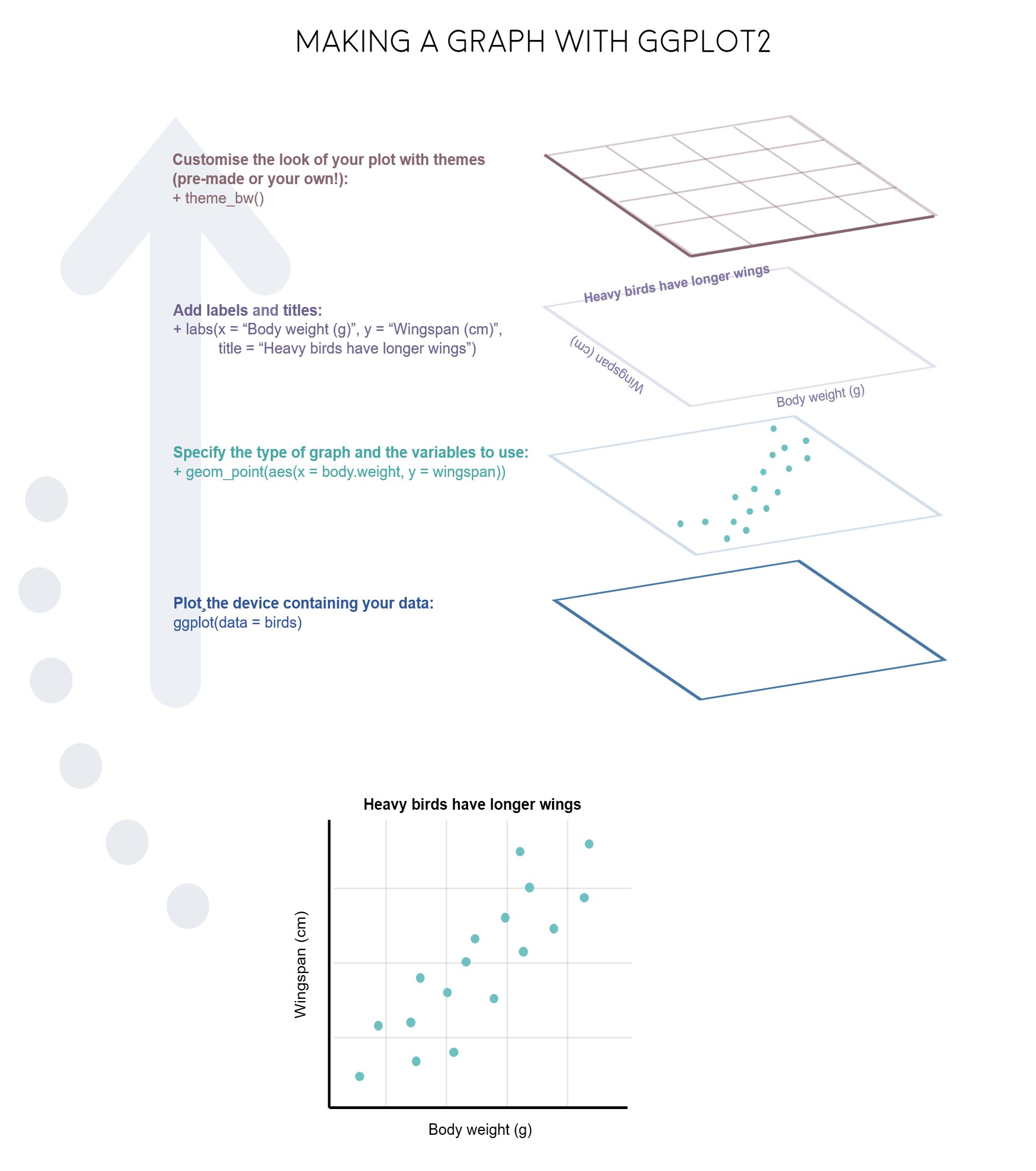
The Grammar of Graphics

ggplot2 is built on the grammar of graphics, a structured system for describing graphs
Every plot is created from the same components:
- data
- aesthetic mappings
- geometric objects (geoms)
- optional: facets, scales, themes, statistics
To load ggplot2 package to the current R environment

library(ggplot2)

1 Scatter Plot: The Basic Structure

ggplot(data = penguins) +
  geom_point(mapping = aes(x = bill_length_mm, y = flipper_length_mm))

How a ggplot is built

ggplot(data = penguins) +
  geom_point(mapping = aes(x = bill_length_mm, y = flipper_length_mm))

`ggplot(data = penguins)`

Creates an empty coordinate system to which multiple layers can be added.
All ggplot2 visualizations begin with the ggplot() function.
The argument data specifies the data frame used for the plot.
Additional layers are added using the plus sign.

`geom_point`

Geometric objects (called geom) are the shapes we put on a plot (e.g. points, bars, etc.).
You can have an unlimited number of layers, but at a minimum a plot must have at least one geom
- geom_point() makes a scatter plot by adding a layer of points.
- geom_line() adds a layer of lines connecting data points.
- geom_col() adds bars for bar charts.
- geom_histogram() makes a histogram.
- geom_boxplot() adds boxes for boxplots

`mapping = aes()`

Each type of geom usually has a required set of aesthetics to be set. Aesthetic mappings are set with the aes() function. Examples include
- x and y (the position on the x and y axes)
- color (“outside” color, like the line around a bar)
- fill (“inside” color, like the color of the bar itself)
- shape (the type of point, like a dot, square, triangle, etc.)
- linetype (solid, dashed, dotted etc.)
- size (of geoms)

Adding labels and themes

ggplot(data = penguins) +
  geom_point(mapping = aes(x = bill_length_mm, y = flipper_length_mm)) +
  labs(
    x = "Bill length",
    y = "Flipper length",
    title = "Scatter plot of bill and flipper length",
    caption = "R package palmerpenguins"
  ) +
  theme_bw()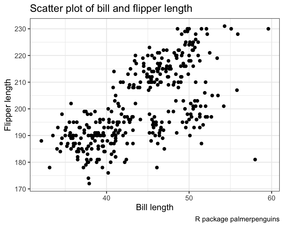

Aesthetic Properties in `ggplot2`

Variables can be linked to a graph through many aesthetic properties in ggplot2.
The most commonly used aesthetics are:
- colors (color, fill)
- shapes and lines (shape, linetype)
- size (size, linewidth)
- transparency (alpha)
- group structure (group)
- position adjustments (x, y)
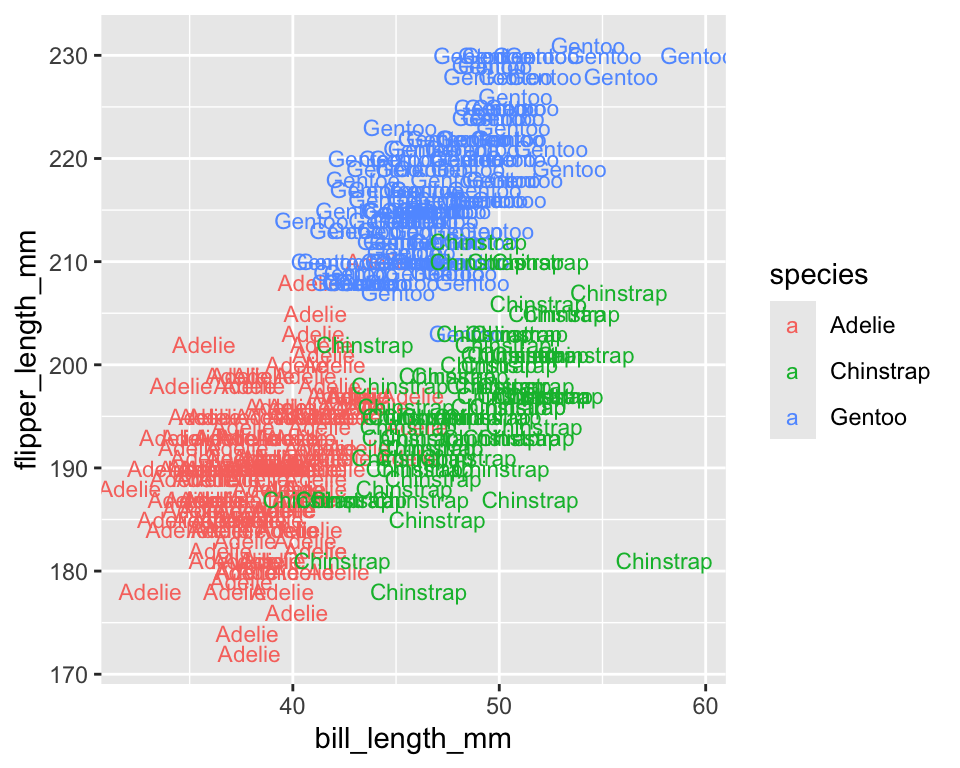
- text aesthetics (label, family, fontface)
- point-specific (stroke)
- bar-specific (width)
Each aesthetic controls a visual aspect of the plot and can be mapped to a variable inside aes().

color controls the outside color of points, lines, and borders
Here different colors represent different levels of species

ggplot(penguins) +
  geom_point(aes(x = bill_length_mm,
                 y = flipper_length_mm,
                 color = species))

fill controls the inside color of shapes such as bars and boxes
Works mainly with geoms that have area (bars, boxes, densities)

ggplot(penguins) +
  geom_boxplot(aes(x = species, y = body_mass_g, fill = species))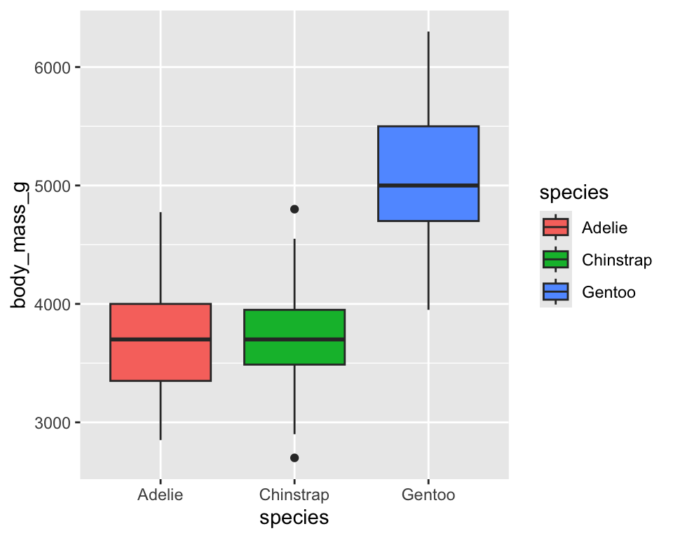

shape assigns different point symbols
ggplot supports up to six distinct shapes for categorical variables

ggplot(penguins) +
  geom_point(aes(x = bill_length_mm,
                 y = flipper_length_mm,
                 shape = species))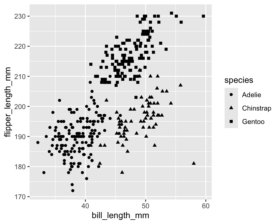

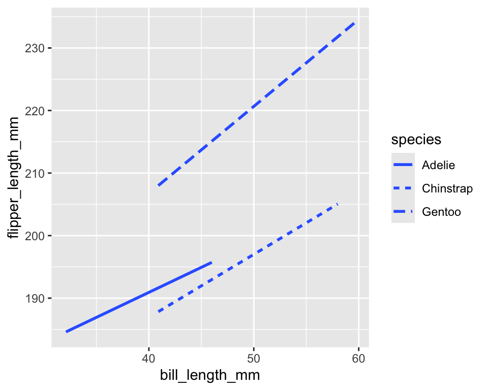
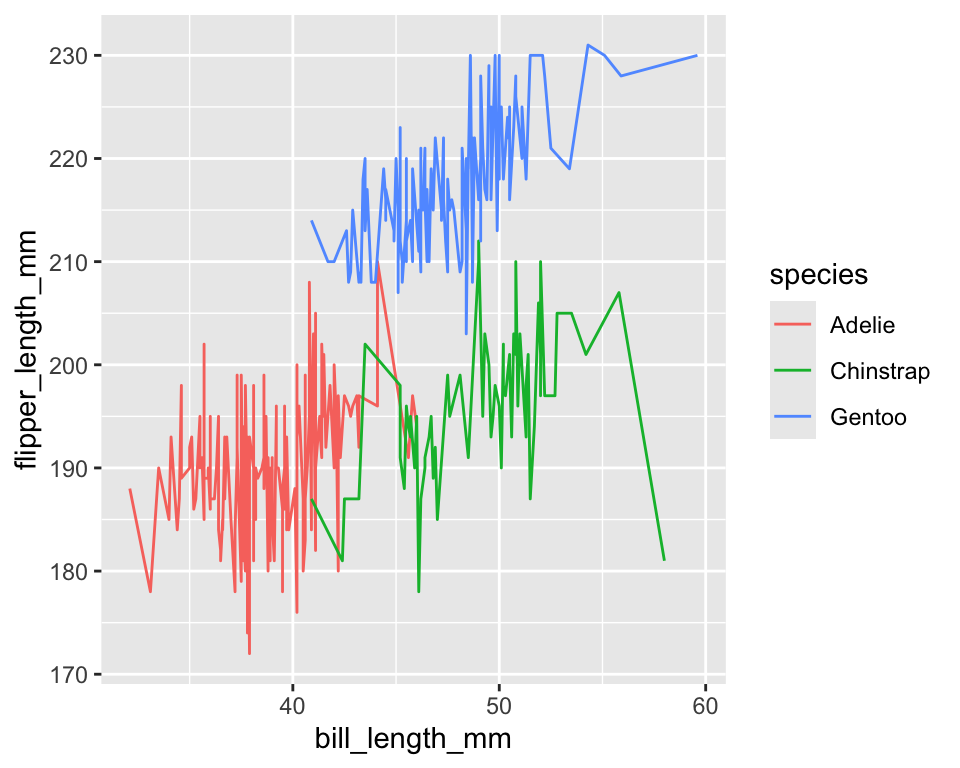
geom_smooth() fits the relationship between two quantitative using a smoothing method
linetype controls solid, dashed, dotted patterns
Useful for distinguishing groups in line plots

ggplot(penguins) +
  geom_smooth(
    aes(x = bill_length_mm, y = flipper_length_mm, linetype = species),
    method = "lm",
    se = FALSE
  )

size controls point size

ggplot(penguins) +
  geom_point(aes(x = bill_length_mm,
                 y = flipper_length_mm,
                 size = body_mass_g))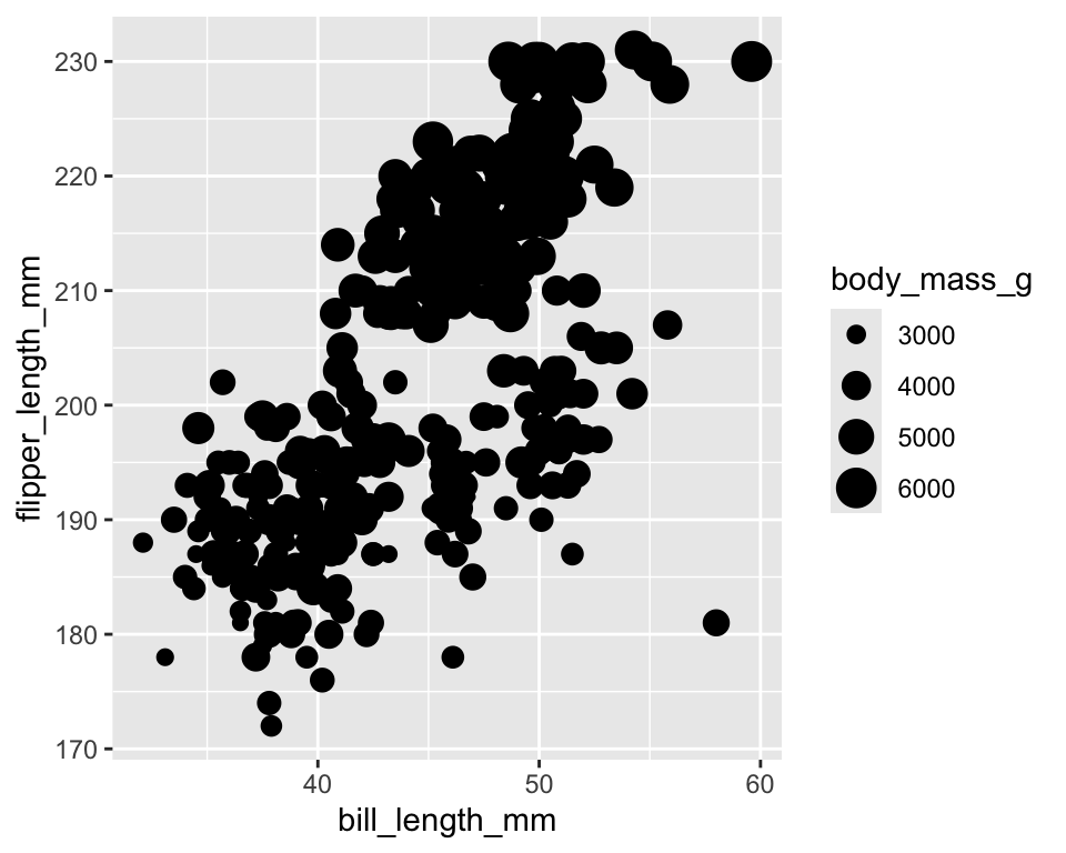

alpha controls transparency (0 = invisible, 1 = opaque)
Useful when points overlap

ggplot(penguins) +
  geom_point(aes(x = bill_length_mm,
                 y = flipper_length_mm,
                 alpha = species))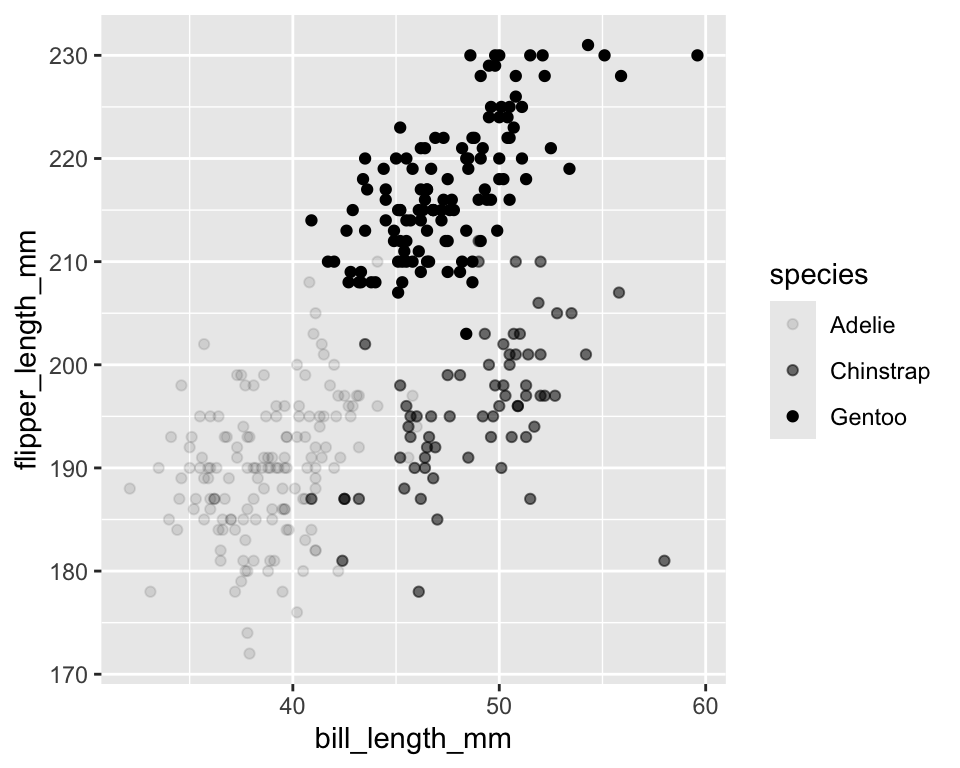

group tells ggplot which observations belong together
Essential for lines, paths, and summaries across categories

ggplot(penguins) +
  geom_line(aes(x = bill_length_mm,
                y = flipper_length_mm,
                group = species,
                color = species))

label is used by text-based geoms
Displays variable values as annotations

ggplot(penguins) +
  geom_text(aes(x = bill_length_mm,
                y = flipper_length_mm,
                label = species,
                colour = species),
  size = 3
  )

How to know which aesthetics work with a geom?

Open the help page: ?geom_point
Use keyboard Tab completion inside aes() to see suggestions

Setting vs Mapping aesthetics

When an aesthetic is inside aes(), it is mapped to a variable
When it is outside aes(), it is set to a constant value

# Mapping (data driven)
ggplot(penguins) +
  geom_point(aes(bill_length_mm, flipper_length_mm, color = species))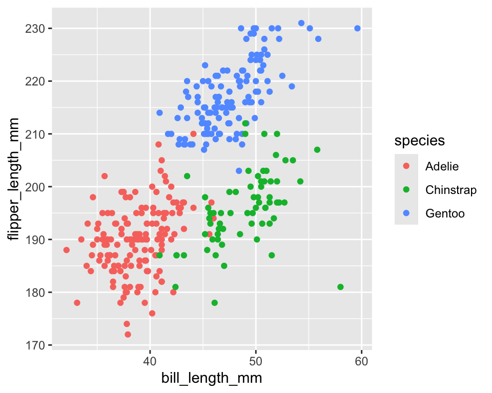

# Setting (fixed appearance)
ggplot(penguins) +
  geom_point(aes(bill_length_mm, flipper_length_mm), color = "blue")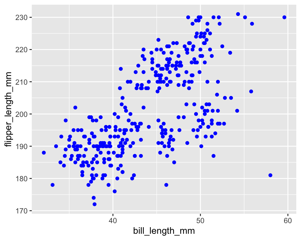

Exercise 3.2.3

(use diamonds data to answer the followings)

Create a scatter plot to examine the effect of price on carat and assign different colors to different levels of cut
Show a fit of a linear model on the scatter plot of carat and price
Show different fits of linear models (price on carat) corresponding to different levels of cut on the scatter plot of price and carat

2 Histogram

geom_histogram() is for histogram
Only x value is needed for its aes() function

ggplot(penguins) +
      geom_histogram(aes(x = body_mass_g))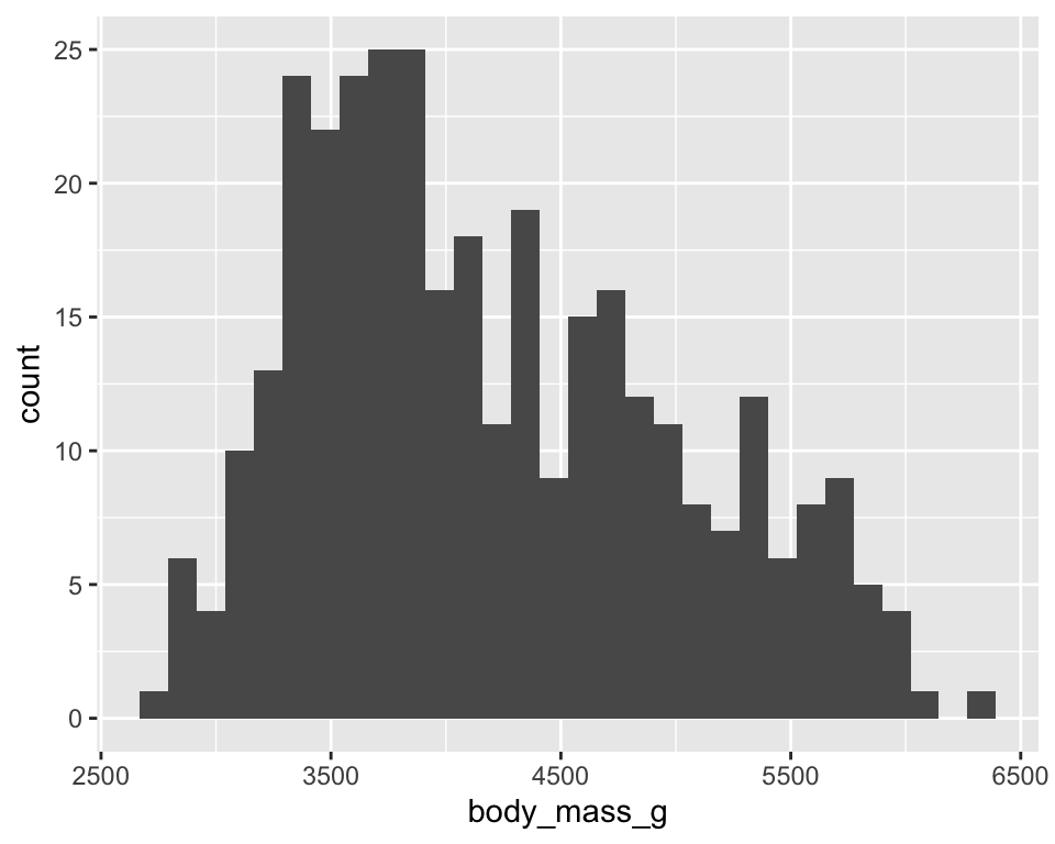

Histogram and density function

geom_density() is used to obtain the density of a variable

ggplot(penguins) +
  geom_histogram(aes(x = body_mass_g, y = after_stat(density)))  +
  geom_density(aes(x = body_mass_g, y = after_stat(density)))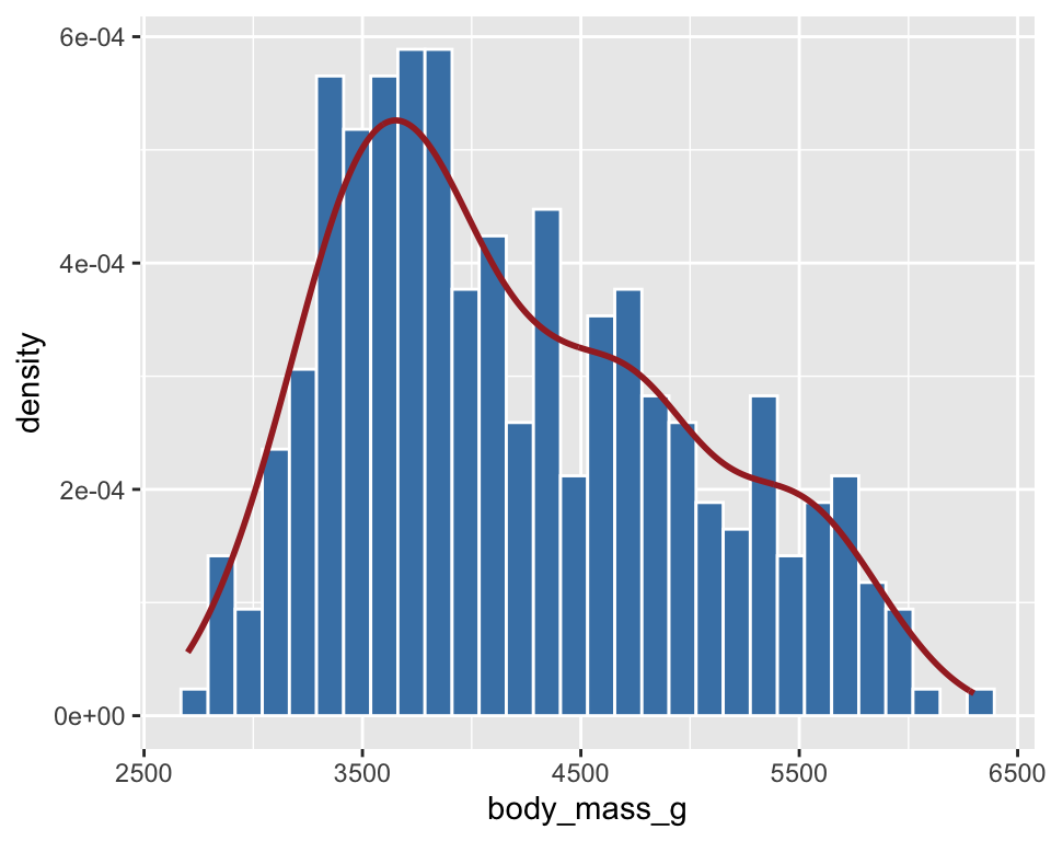

A common mapping function in ggplot() for different geom_*()

ggplot(penguins, aes(x = body_mass_g, y = after_stat(density))) +
  geom_histogram(fill = "steelblue", color = "white") +
  geom_density(color = "brown", size = 1)

Exercise 3.2.1

(use diamonds data to answer the followings)

Create a histogram of carat and check the effect of bins on histogram
Add a density line to the plot obtained in Question 1

3 Boxplot

`geom_boxplot()`

ggplot(penguins) +
  geom_boxplot(aes(x = species, y = body_mass_g))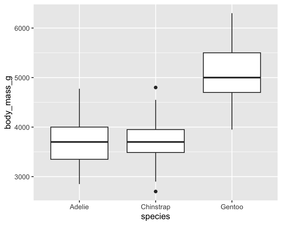

ggplot(penguins) +
  geom_boxplot(aes(x = species, y = body_mass_g), fill = "brown") +
  coord_flip()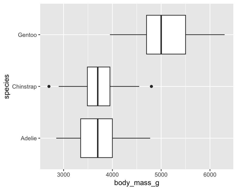

Boxplot with original data points

ggplot(penguins, aes(x = species, y = body_mass_g)) +
  geom_boxplot() +
  geom_jitter(width = .2, aes(color = species), size = .75)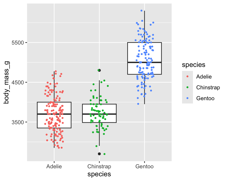

geom_jitter() adds a small amount random variation to each point and it is useful to visualize points at different levels

Exercise 3.2.2

(use diamonds data to answer the followings)

Create a boxplot of carat at different levels of cut
Create a scatter plot to examine the effect of carat on price

Facets

Sometimes a plot becomes crowded when too many variables are shown using colors or shapes.
Facets display additional categorical variables by splitting a plot into multiple smaller panels, one for each group.
ggplot2 provides two main functions for faceting:
- facet_wrap() → splits the plot by one categorical variable
- facet_grid() → splits the plot by two categorical variables arranged in rows and columns

Faceting allows us to compare patterns across groups while keeping the same axes and scales.

ggplot(penguins) +
  geom_point(aes(x = flipper_length_mm, y = bill_length_mm)) +
  facet_wrap(~species)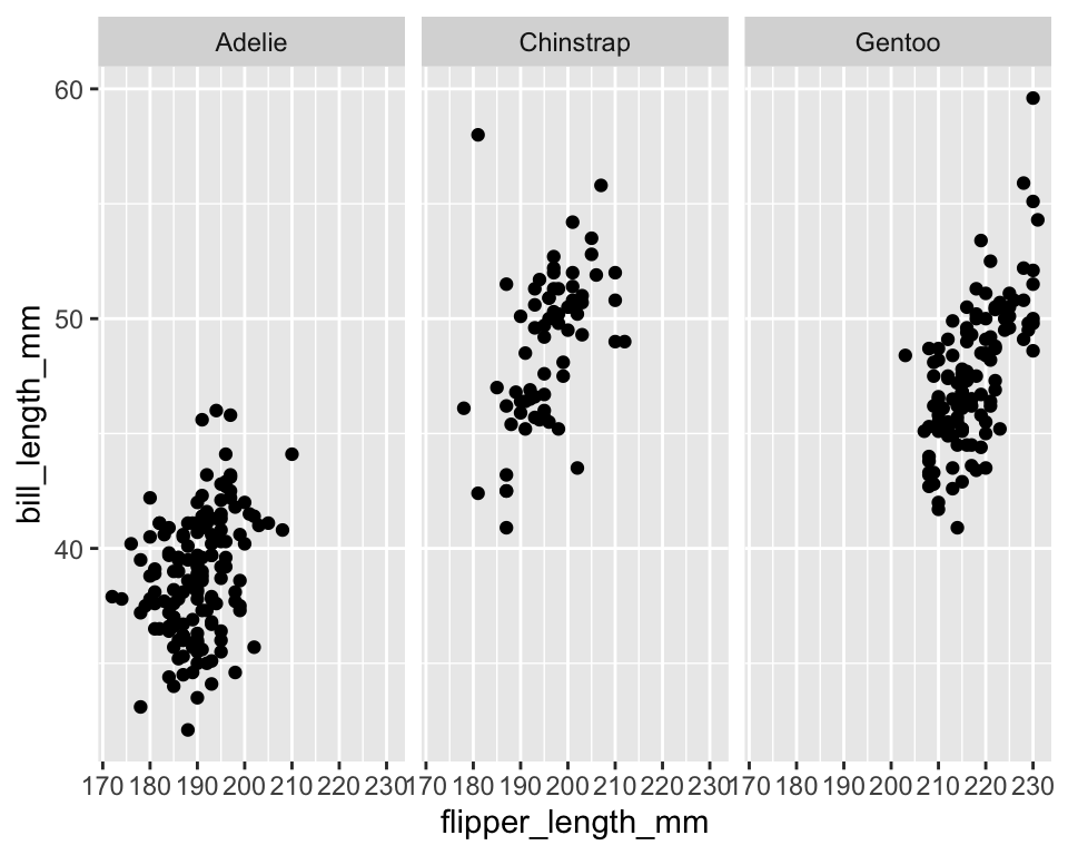

ggplot(penguins,
       aes(x = flipper_length_mm, y = bill_length_mm, color = species)) +
  geom_point() +
  geom_smooth(method = "lm", se = FALSE, color = "black") +
  facet_wrap(~species)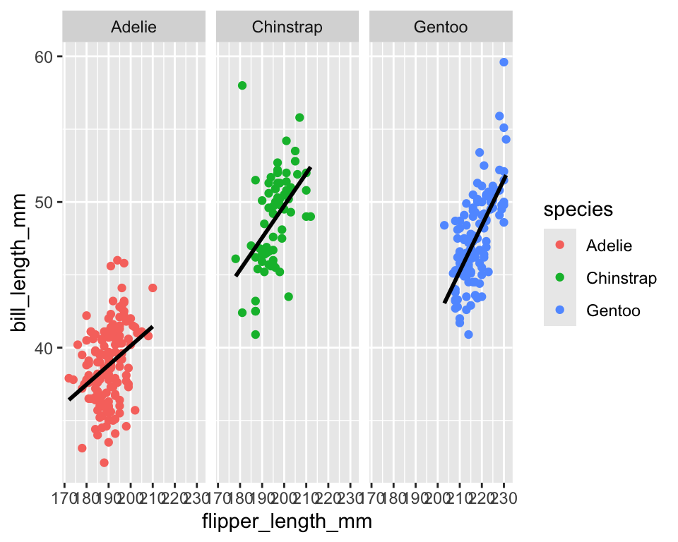

ggplot(data = penguins[!is.na(penguins$sex), ]) +
  geom_point(aes(x = flipper_length_mm, y = bill_length_mm)) +
  facet_wrap(~ sex + species)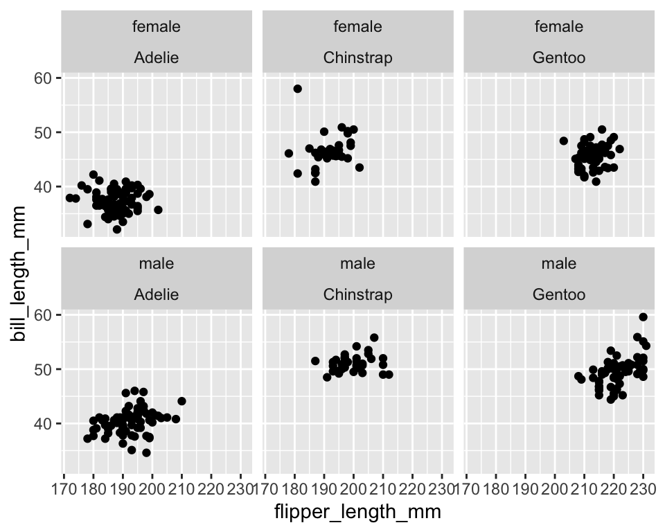

ggplot(data = penguins[!is.na(penguins$sex), ]) +
  geom_point(aes(x = flipper_length_mm, y = bill_length_mm)) +
  facet_grid(sex ~ species)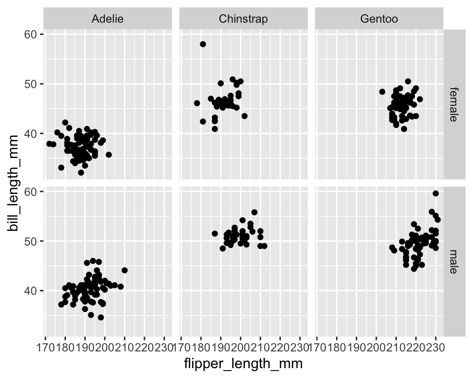

ggplot(penguins) +
  geom_histogram(aes(x = body_mass_g),
                 color = "brown",
                 fill = "yellow") +
  facet_wrap(~ species, ncol = 1)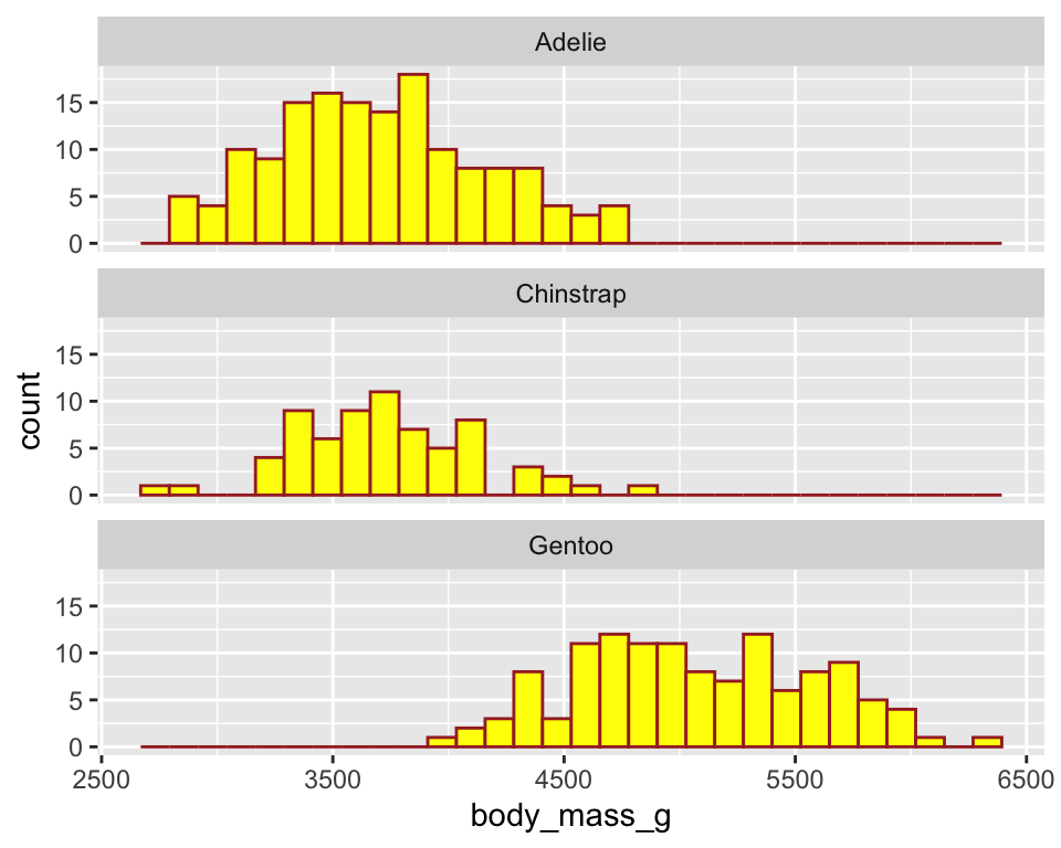

ggplot(penguins) +
  geom_histogram(aes(x = body_mass_g),
                 color = "brown",
                 fill = "yellow") +
  facet_wrap(~ species, ncol = 1) +
  theme_minimal()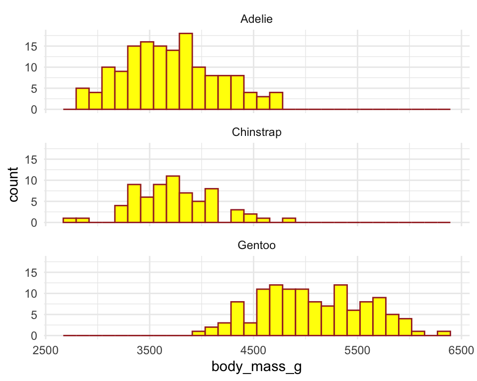

ggplot(penguins) +
  geom_histogram(aes(x = body_mass_g),
                 color = "brown",
                 fill = "yellow") +
  facet_wrap(~ species, ncol = 1) +
  theme_minimal() +
  theme(panel.grid = element_blank())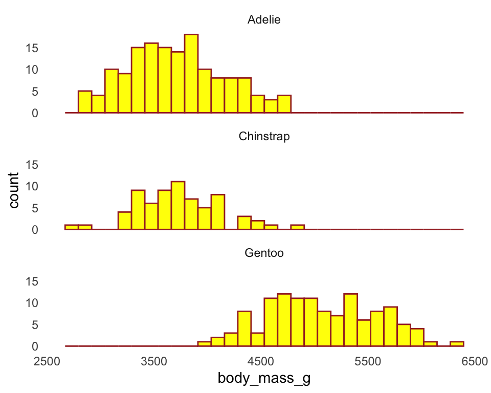

Exercise 3.2.4

(use diamonds data to answer the followings)

Create histogram of x at different levels of cut

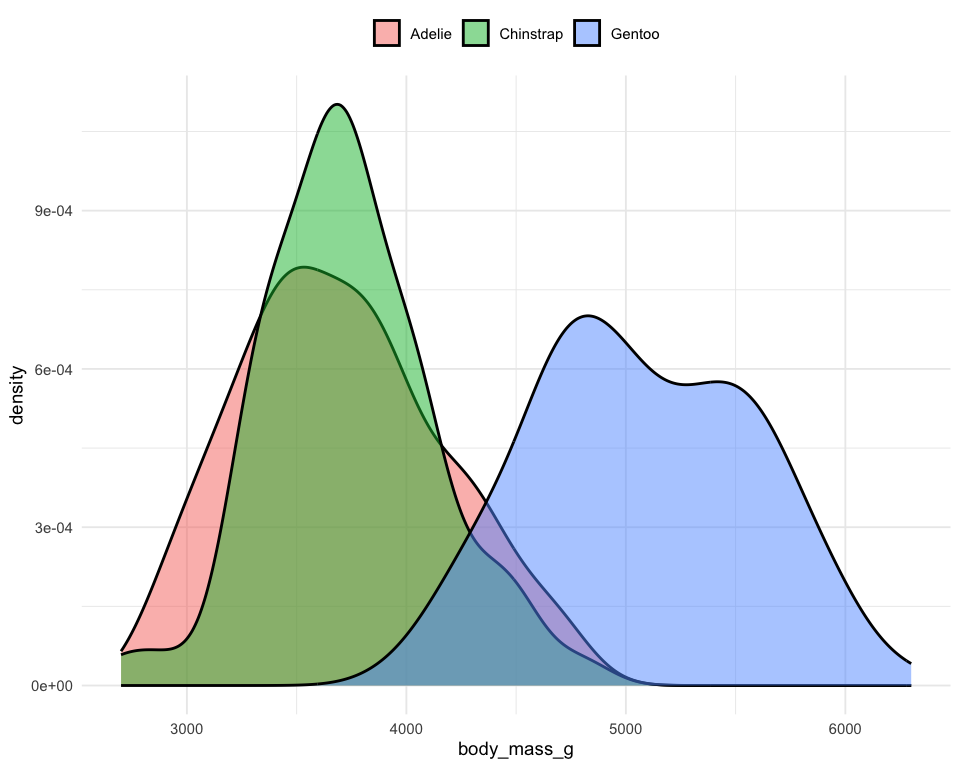
4 Density plot

Distribution of penguins’ body mass

ggplot(penguins) +
  geom_density(aes(x = body_mass_g, fill = species), alpha = .5)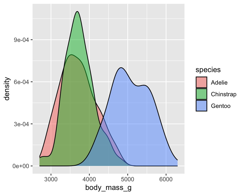

Density plot

Distribution of penguins’ body mass

ggplot(penguins) +
  geom_density(aes(x = body_mass_g, fill = species), alpha = .5) +
  theme(legend.position = "top", legend.title = element_blank())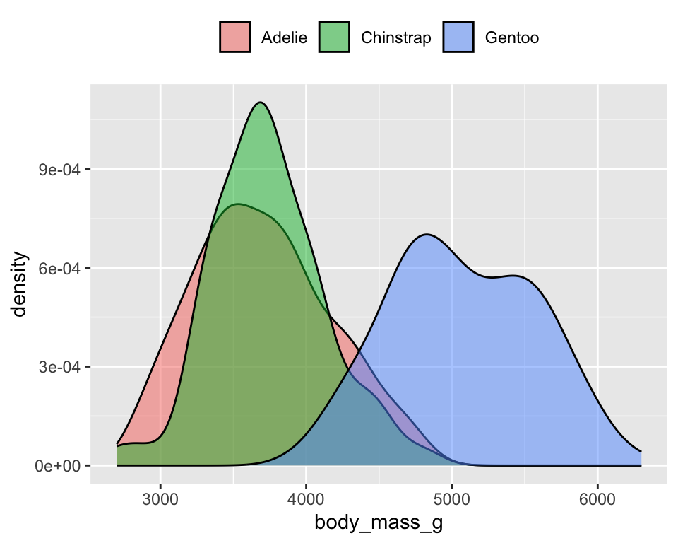

Distribution of penguins’ body mass

ggplot(penguins) +
  geom_density(aes(x = body_mass_g, fill = species), alpha = .5) +
  theme_minimal(base_size = 7) +
  theme(legend.position = "top", legend.title = element_blank())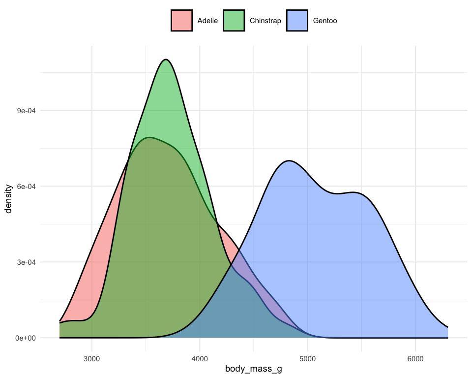

Distribution of penguins’ body mass

ggplot(penguins) +
  geom_density(aes(x = body_mass_g, fill = species), alpha = .5) +
  theme_minimal(base_size = 7) +
  theme(
    legend.position = "top",
    legend.key.size = unit(.75, "lines"),
    legend.title = element_blank()
  )

5 Bar Chart

Frequency bar chart

Frequency distribution of penguin species

ggplot(penguins) +
  geom_bar(aes(x = species), fill = "steelblue")

Value bar chart (mean)

Mean Body Mass by Species

penguins |>
  group_by(species) |>
  summarise(mean_mass = mean(body_mass_g, na.rm=T)) |>
  ggplot(aes(x = species, y = mean_mass)) +
  geom_col(fill = "steelblue")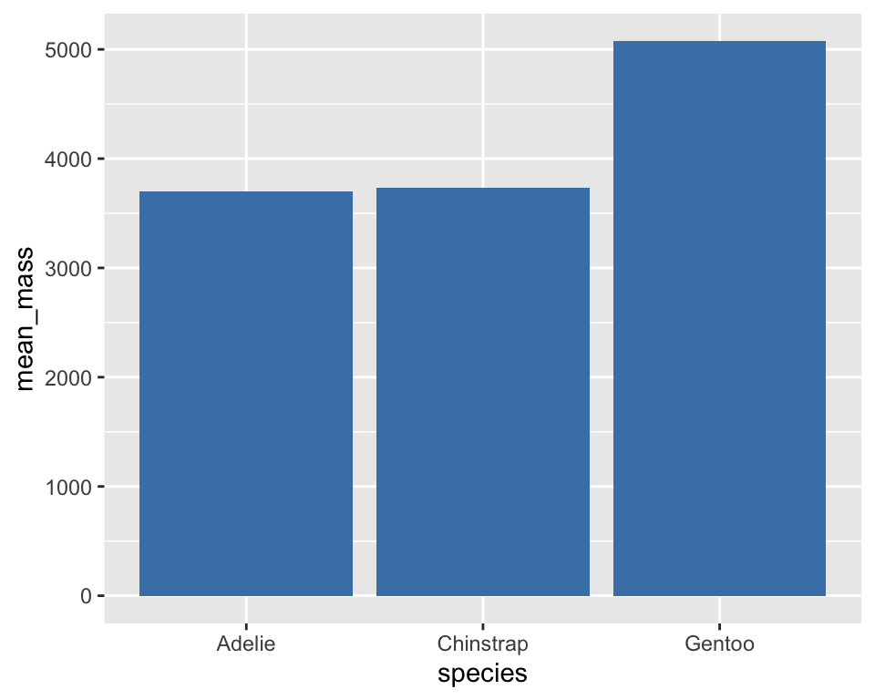

geom_col() creates a bar chart where bar heights come from a variable, while geom_bar() creates a bar chart based on frequencies.

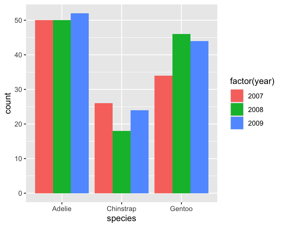
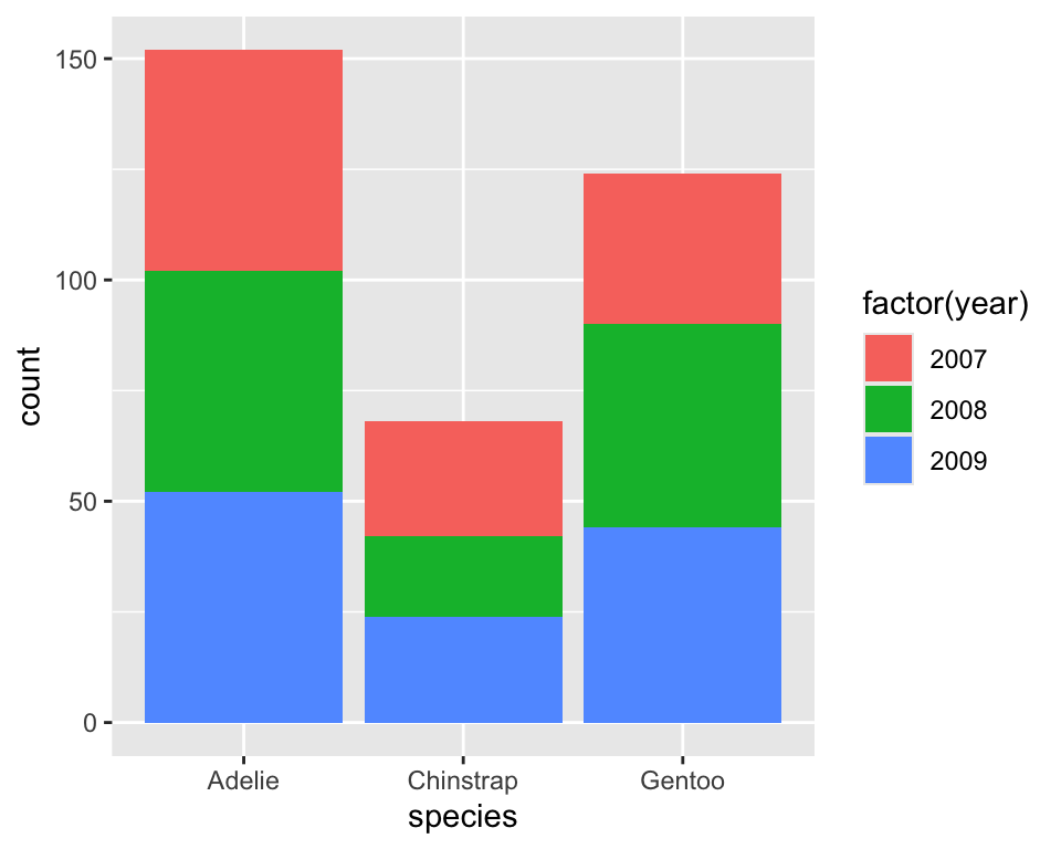
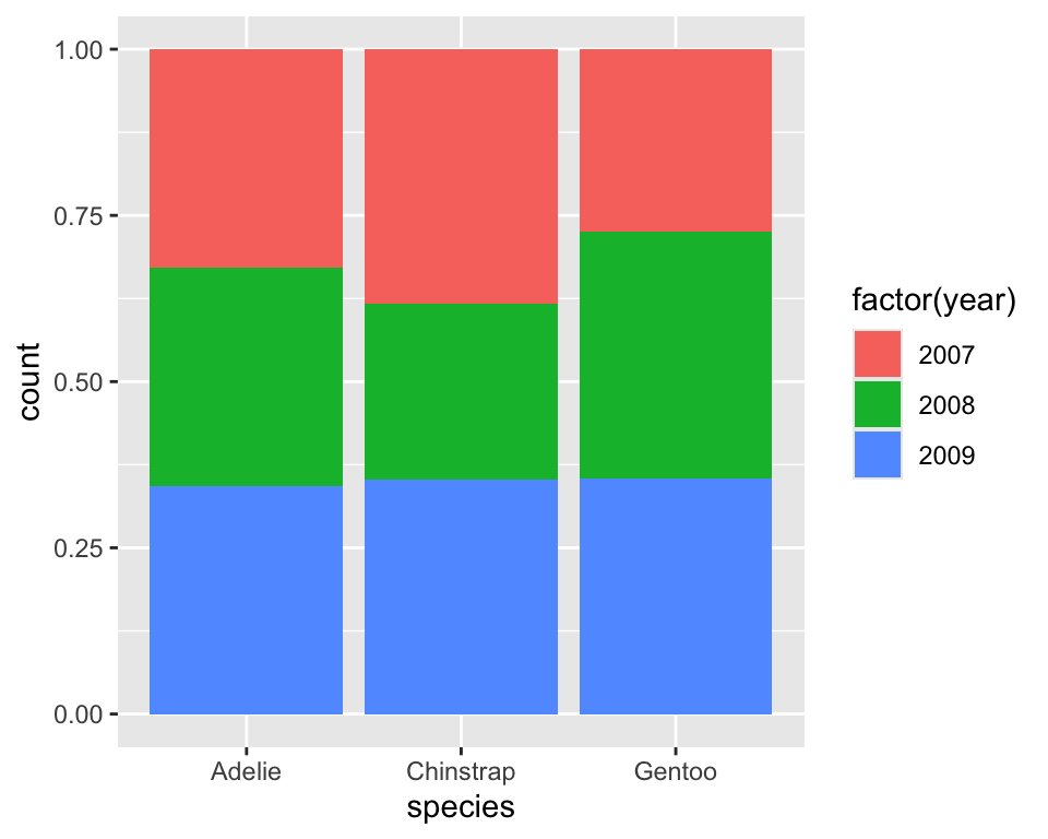
Frequency barchart with two variables

Distribution of species by year

ggplot(penguins) +
  geom_bar(aes(x = species, fill = factor(year)), position = "dodge")

ggplot(penguins) +
  geom_bar(aes(x = species, fill = factor(year)), position = "stack")

ggplot(penguins) +
  geom_bar(aes(x = species, fill = factor(year)), position = "fill")

Exercise 3.2.5

(use diamonds data to answer the followings)

Create a barplot of cut
Create a barplot of color
Create a barplot of cut with showing the distribution of color at different levels of cut
Check the use three different value of the argument position when creating a barplot with cut and color

Homework

Use the package gapminder to get an access to the data gapminder
gapminder has 6 variables and 1704 observations, where the variables are:

#> [1] "country"   "continent" "year"      "lifeExp"   "pop"       "gdpPercap"

Create a scatter plot to examine how gdpPercap affects lifeExp
Change the scale of x-axis to log base 10
Add a color layer corresponding to continent to the previous graph

Create a scatter plot of gdpPercap versus lifeExp for different continents in different plotting regions
Add smooth lines to describe relationship between gdpPercap and lifeExp for different continents separately
Draw a boxplot of lifeExp to compare distribution life expectancy for different continents
Draw a histogram of lifeExp and check it shapes for different bin size
Draw density plots of lifeExp for different continents in a single plot

Make a scatter plot of lifeExp on the y-axis against year on the x
Fit a straight line to estimate mean life expectancy for a year for different countries
Split the plot for different continents
Add a continent-specific mean line to the plot

Statistical layers `geom_()` vs `stat_()`

In ggplot2, every geom is linked to a statistic.
Each geom has a default stat, and each stat has a default geom.

Example: smoothing

# The following codes produce the same result.
ggplot(penguins, aes(bill_length_mm, flipper_length_mm)) +
  geom_smooth(stat = "smooth")

ggplot(penguins, aes(bill_length_mm, flipper_length_mm)) +
  stat_smooth(geom = "smooth")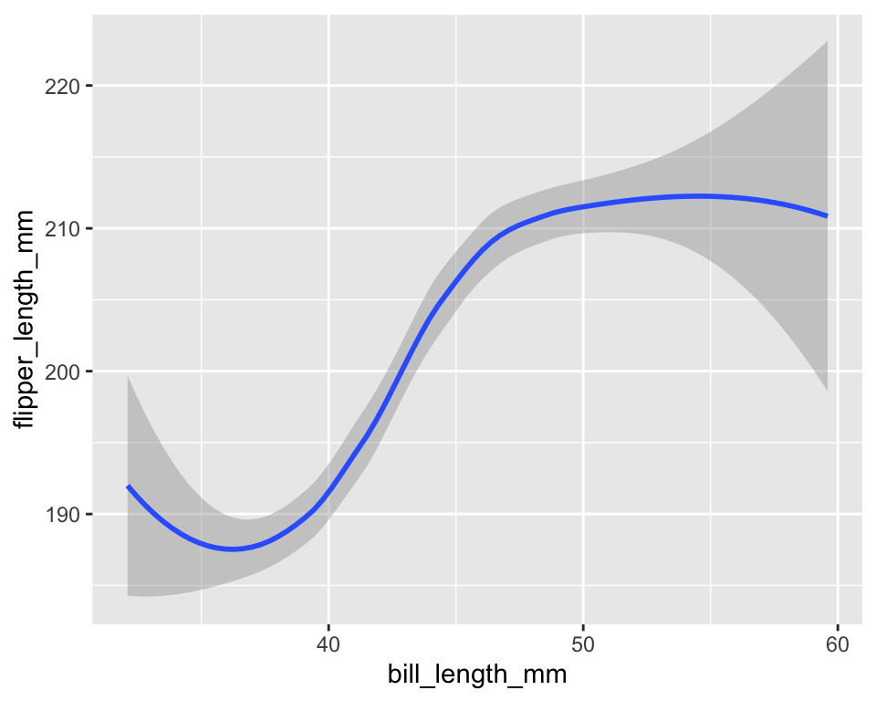

Example: identity stat for points

# The following codes produce the same result.
ggplot(penguins, aes(bill_length_mm, flipper_length_mm)) +
  geom_point(stat = "identity")

ggplot(penguins, aes(bill_length_mm, flipper_length_mm)) +
  stat_identity(geom = "point")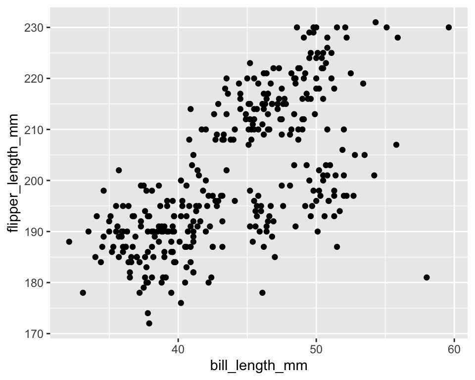

Example: counting for bar charts

# The following codes produce the same result.
ggplot(penguins, aes(species)) +
  geom_bar(stat = "count")

ggplot(penguins, aes(species)) +
  stat_count(geom = "bar")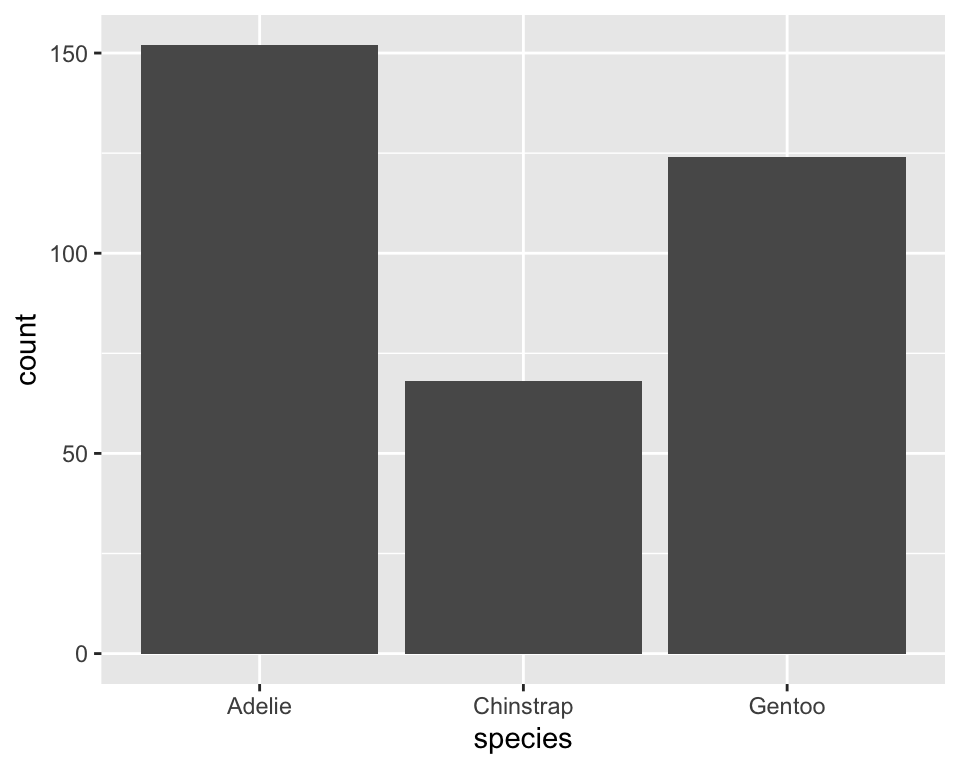

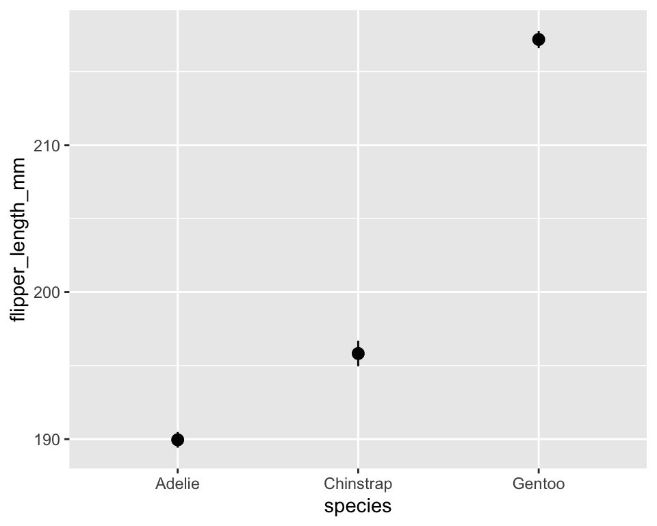
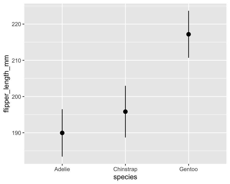
Statistical summaries

stat_summary() allows us to display custom summaries instead of raw data.

# The following codes produce the same result.
ggplot(penguins, aes(species, flipper_length_mm)) +
  stat_summary()

ggplot(penguins, aes(species, flipper_length_mm)) +
  stat_summary(fun.data = mean_se, geom = "pointrange")

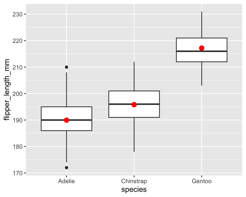
Adding summaries to existing geoms

ggplot(penguins, aes(species, flipper_length_mm)) +
  geom_boxplot() +
  stat_summary(
    fun = mean,
    geom = "point",
    color = "red",
    size = 3
  )

Mean Body Mass by Species

ggplot(penguins, aes(x = species, y = body_mass_g)) +
  stat_summary(fun = mean, geom = "col", fill = "steelblue")

Custom summary functions

ggplot(penguins, aes(species, flipper_length_mm)) +
  stat_summary(
    fun = mean,
    fun.max = function(y) mean(y) + sd(y),
    fun.min = function(y) mean(y) - sd(y)
  )

Data vizualization with ggplot2

Why ggplot2?

The Grammar of Graphics

1 Scatter Plot: The Basic Structure

How a ggplot is built

ggplot(data = penguins)

geom_point

mapping = aes()

Adding labels and themes

Aesthetic Properties in ggplot2

How to know which aesthetics work with a geom?

Setting vs Mapping aesthetics

Exercise 3.2.3

2 Histogram

Histogram and density function

Exercise 3.2.1

3 Boxplot

geom_boxplot()

Boxplot with original data points

Exercise 3.2.2

Facets

Exercise 3.2.4

4 Density plot

Density plot

5 Bar Chart

Frequency bar chart

Value bar chart (mean)

Frequency barchart with two variables

Exercise 3.2.5

Homework

Statistical layers geom_*() vs stat_*()

Example: smoothing

Example: identity stat for points

Example: counting for bar charts

Statistical summaries

Adding summaries to existing geoms

Mean Body Mass by Species

Custom summary functions

Data vizualization with `ggplot2`

`ggplot(data = penguins)`

`geom_point`

`mapping = aes()`

Aesthetic Properties in `ggplot2`

`geom_boxplot()`

Statistical layers `geom_()` vs `stat_()`