4 Data Structures in R
1 Data in R
Until now, you’ve created fairly simple data in R and stored it as a vector.
However, most (if not all) of you will have much more complicated datasets from your various experiments and surveys that go well beyond what a vector can handle.
In previous lectures we’ve gone through the main four data types (i.e vector types) in R, i.e. logical, integer, double, character
Now let’s have a look at some of main structures that we have for storing these data.
2 Data Structures
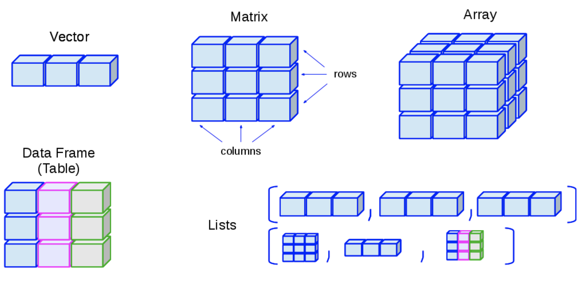
- R has many data structures, some of the important ones are:
1. Atomic vectors
2. Matrices
3. Arrays
4. Factors
5. Lists
6. Data frames
7. Tibbles
3 Atomic Vectors
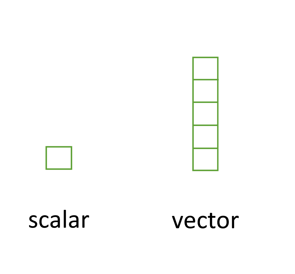
- Perhaps the simplest type of data structure is the vector
- You’ve already been introduced to vectors
- Vectors that have a single value (length 1) are called scalars
- key thing to remember is that all the elements inside a vector must be of the same data type
4 Matrices
When a rectangular data structure contains a single type of data in all its cells (i.e., in all its rows and columns), we have a matrix of data.
In R, a matrix really is an atomic vector that is tweaked into another shape (i.e., a re-shaped vector).
Internally, this is implemented by taking a vector and adding attributes that describe its shape and the names of its rows or columns
- R function
matrix()is used to create a matrix from a atomic vector.
matrix(1:6, nrow = 2) # default: byrow = FALSE
#>      [,1] [,2] [,3]
#> [1,]    1    3    5
#> [2,]    2    4    6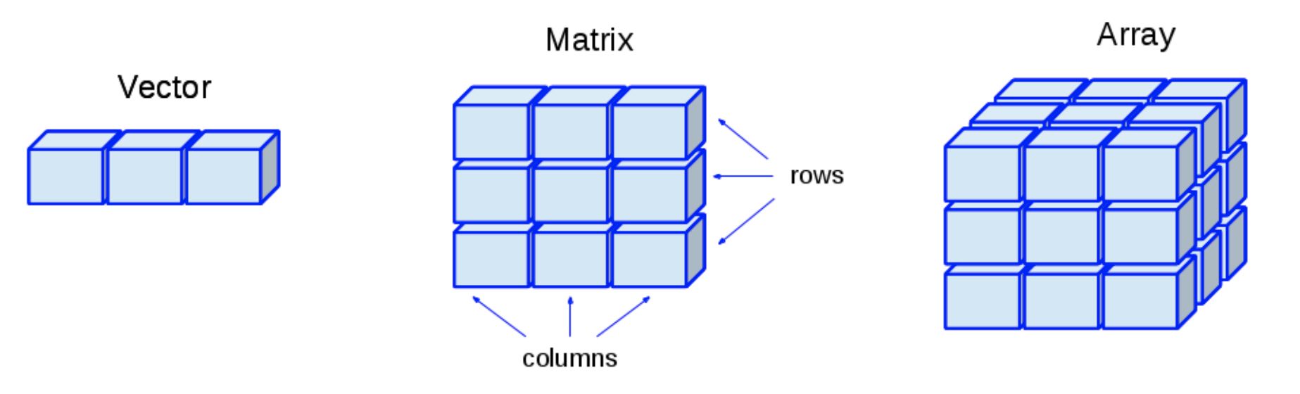
5 Arrays
- Arrays are just multidimensional matrices
Summary:
- Like vectors and matrices, arrays must contain elements all of the same data types.
- Data structures like matrices, or arrays are built on top of atomic vectors by adding attributes
- In other words, matrices and arrays are just atomic vectors with a
dim()(dimension) attribute
6 Calculations on matrices
- Sometimes it’s also useful to define row and column names for your matrix
- The usual matrix addition, multiplication etc can be performed. Note the use of the
%*%operator to perform matrix multiplication.
# element by element products
mat1 * mat2
#>      [,1] [,2]
#> [1,]    2    0
#> [2,]    0    2
# matrix multiplication
mat1 %*% mat2
#>      [,1] [,2]
#> [1,]    3    2
#> [2,]    1    2
7 Basic martrix functions
R has numerous built in functions to perform matrix operations
For example, to transpose a matrix we use the transposition function
t()
my_mat_t <- t(my_mat)
my_mat_t
#>   A B  C  D
#> a 1 5  9 13
#> b 2 6 10 14
#> c 3 7 11 15
#> d 4 8 12 16- To extract the diagonal elements of a matrix and store them as a vector we can use the
diag()function.
my_mat_diag <- diag(my_mat)
my_mat_diag
#> [1] 1 6 11 16| Functions | Description |
|---|---|
chol(x) |
Choleski decomposition |
t(x) |
Transpose of a matrix \(x\). |
diag(x) |
Extracts the diagonal elements of a matrix |
ncol(x) |
Returns the number of columns |
nrow(x) |
Returns the number of rows |
colSums(x) |
Returns the sum of columns |
rowSums(x) |
Returns the sum of rows |
solve(A,b) |
Solve the system \(A x=b\) |
solve(x) |
Calculate the inverse |
8 Exercise 4
Create a vector called
xconsisting of the first fifteen integers of the number line.Use the function
dim()to assign dimension to vectorxwith three rows and five columns. What is the class ofxnow?Given the following matrices, \[ A=\left[\begin{array}{llll} 2 & 9 & 0 & 0 \\ 0 & 4 & 1 & 4 \\ 7 & 5 & 5 & 1 \\ 7 & 8 & 7 & 4 \end{array}\right] \quad b=\left[\begin{array}{c} -1 \\ 6 \\ 0 \\ 9 \end{array}\right] \]
- Calculate \(A^T b\).
- Find the inverse of matrix \(A\).
- Solve the equation for \(x\), where \(A x=b\).
Generate a vector
x0of order 20 with all elements as 1Generate a vector
x1of order 20 with elements randomly selected from 30:70, consider a seed 80Create a matrix
Xwith the first columnx0and the second columnx1Generate a vector
Yof order 20 using the equation \(y_i = 1.2 + 1.8x1 + \epsilon_i,\) where \(\epsilon_i\sim N(0, 9)\)Obtain the value of \((X'X)^{-1}X'Y\), use the R function
solve()to obtain an inverse of a square matrix.
9 S3 Atomic Vectors:
-
R objects can carry different attributes, such as:
-
names→ names of elements in a vector -
dim→ dimensions of a matrix or array -
class→ tells R how to treat the object
-
Adding a class attribute makes an object part of the S3 object system.
This means that the object will behave differently when passed to generic functions like
print(),summary(), orplot().Every S3 object is built on top of a base type, and often stores additional information in other attributes
-
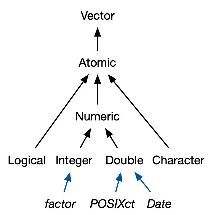
Many important base R data types are actually S3 objects built on atomic vectors:
-
Factors → built on top of integer vectors with
levelsandclass = "factor" -
Dates → built on top of double vectors with
class = "Date" -
Date-times → built on top of double vectors with
class = "POSIXct"orclass = "POSIXlt"
-
Factors → built on top of integer vectors with
These are sometimes called S3 atomic vectors because they are still vectors at their core, but their
classattribute gives them new behavior.Among these, we will discuss only the
factorvector.
10 Factors
Factors are used to store categorical information in R, a categorical variable has only pre-defined levels, e.g., gender has two levels
maleandfemaleFactors are similar to
characterdata except it can take only predefined values-
Factors are built on top of an integer vector with two attributes:
-
factor→ which makes it behave differently from regular integer vectors, and -
levels→ which defines the set of allowed value
-
Factors look like strings, but behave like integers
-
The function
factor()is used to create factor vector from an atomic vector and it has the following arguments-
x\(\rightarrow\) data vector -
levels\(\rightarrow\) values ofxthat will be used as the level of the factor -
labels\(\rightarrow\) a vector of labels for the levels
-
# Creating factor using factor()
fac = factor(x = c(1, 2, 1, 1, 2, 1, 2),
              levels = c(1, 2),
              labels = c("Male", "Female"))
fac
#> [1] Male   Female Male   Male   Female Male   Female
#> Levels: Male Female
as.character(fac)
#> [1] "Male"   "Female" "Male"   "Male"   "Female" "Male"   "Female"
# not providing levels
fac1 = factor(c("Male", "Female", "Male",
"Male", "Female", "Male", "Female"))
fac1
#> [1] Male Female Male Male Female Male Female
#> Levels: Female Male
# providing levels
fac2 = factor(c("Male", "Female", "Male",
"Male", "Female", "Male", "Female"),
levels = c("Male", "Female"))
fac2
#> [1] Male Female Male Male Female Male Female
#> Levels: Male Femaletypeof(fac1)
#> [1] "integer"
attributes(fac1)
#> $levels
#> [1] "Female" "Male"
#>
#> $class
#> [1] "factor"11 Lists
List is a vector with heterogeneous elements, i.e., each element of a list can be any type
The function
list()is used to create a list
str(list1)
#> List of 4
#>  $ : int [1:3] 1 2 3
#>  $ : chr "a"
#>  $ : logi [1:3] TRUE FALSE FALSE
#> $ : num [1:3] 2.5 5.1 9- Lists are sometimes called recursive vectors because a list can contain other lists. This makes them fundamentally different from atomic vectors
- List
12 S3 Lists:
Recall: Data structures like matrices, arrays, or factors are built on top of atomic vectors by adding attributes.
-
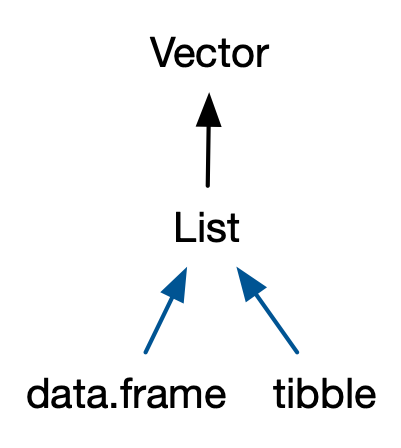
Similarly, in addition to the regular lists, there are two important S3 vectors built on top of lists
- They are are data frames and tibbles.
13 Data Frames
A data frame is a named list of vectors with attributes for (column)
names,row.names, and itsclass, “data.frame”-
In contrast to a regular list, a data frame has an additional constraint:
- the length of each of its vectors must be the same
This gives data frames their rectangular structure
Columns are variables, and rows are observations
Data frame is R’s equivalent to spreadsheet
If you do data analysis in R, you’re going to be using data frames
- R function
data.frame()is used to create a new data frame, where atomic vectors can be used as inputs
# Creating a data frame
name = c("Fahim", "Abir", "Aman")
language = c("R", "Python", "Java")
age = c(22, 25, 45)
df = data.frame(name, language, age)
df
#>    name language age
#> 1 Fahim        R  22
#> 2  Abir   Python  25
#> 3 Aman Java 45typeof(df)
#> [1] "list"
attributes(df)
#> $names
#> [1] "name" "language" "age"
#>
#> $class
#> [1] "data.frame"
#>
#> $row.names
#> [1] 1 2 3- While the attributes of data frame and matrix are different, a matrix can be transformed into a data frame using the function
as.data.frame()
mat1 <- matrix(1:12, nrow = 3)
attributes(mat1)
#> $dim
#> [1] 3 4
mat2 <- as.data.frame(mat1)attributes(mat2)
#> $names
#> [1] "V1" "V2" "V3" "V4"
#>
#> $class
#> [1] "data.frame"
#>
#> $row.names
#> [1] 1 2 3There are various ways to inspect a data frame, such as:
-
str()gives a very brief description of the data -
names()gives the name of each variable in the data -
summary()gives some very basic summary statistics for each variable -
head()shows the first few rows -
tail()shows the last few rows
14 Tibbles
Data frame is one of the most important ideas in R and it is one of the things that make R different from other programming languages
Data frames are created more than 20 years ago and over the years, the way people use R have changed
Some of the design decisions of data frame do not go well with current way of using R
Tibbles are similar to data frames and it overcome some of limitations of data frames
Tibbles are not the part of the base R, it is in the R package
tibbleTo use tibble, one need to load the package
tibbleto the current R environment
# Load the tibble package
library(tibble)
# Create a tibble with three columns: name, age, and city
my_data <- tibble(
  name = c("Samir", "Amir", "Aman"),
  age = c(25, 30, 35),
  city = c("Dhaka", "Khulna", "Jashore")
)
my_data
#> # A tibble: 3 × 3
#>   name    age city
#>   <chr> <dbl> <chr>
#> 1 Samir    25 Dhaka
#> 2 Amir     30 Khulna
#> 3 Aman     35 Jashore
15 Data frame vs. Tibble
Data frame
df2 <- data.frame(
  x = 1:3,
  y = LETTERS[1:3],
  z = c(2, 4, 6)
)
df2
#>   x y z
#> 1 1 A 2
#> 2 2 B 4
#> 3 3 C 6
typeof(df2)
#> [1] "list"Data frame
attributes(df2)
#> $names
#> [1] "x" "y" "z"
#>
#> $class
#> [1] "data.frame"
#>
#> $row.names
#> [1] 1 2 3
str(df2)
#> 'data.frame':    3 obs. of  3 variables:
#>  $ x: int  1 2 3
#>  $ y: chr  "A" "B" "C"
#>  $ z: num  2 4 6
Tibble
attributes(tb2)
#> $class
#> [1] "tbl_df"     "tbl"        "data.frame"
#>
#> $row.names
#> [1] 1 2 3
#>
#> $names
#> [1] "x" "y" "z"
str(tb2)
#> tibble [3 × 3] (S3: tbl_df/tbl/data.frame)
#>  $ x: int [1:3] 1 2 3
#>  $ y: chr [1:3] "A" "B" "C"
#> $ z: num [1:3] 2 4 6- While data frames automatically recycle columns that are an integer multiple of the longest column, tibbles will only recycle vectors of length one
Data frame
data.frame(x = 1:4, y = 1:2)
#>   x y
#> 1 1 1
#> 2 2 2
#> 3 3 1
#> 4 4 2data.frame(x = 1:4, y = 1:3)
#> Error in data.frame(x = 1:4, y = 1:3): arguments imply differing number of rows: 4, 3Tibble
- A data frame
mtcarsis available in base R
head(mtcars, 2)
#>               mpg cyl disp  hp drat    wt  qsec vs am gear carb
#> Mazda RX4      21   6  160 110  3.9 2.620 16.46  0  1    4    4
#> Mazda RX4 Wag  21   6  160 110  3.9 2.875 17.02  0  1    4    4
mtcars_t <- as_tibble(mtcars)
mtcars_t
#> # A tibble: 32 × 11
#> mpg cyl disp hp drat wt qsec vs am gear carb
#> <dbl> <dbl> <dbl> <dbl> <dbl> <dbl> <dbl> <dbl> <dbl> <dbl> <dbl>
#> 1 21 6 160 110 3.9 2.62 16.5 0 1 4 4
#> 2 21 6 160 110 3.9 2.88 17.0 0 1 4 4
#> 3 22.8 4 108 93 3.85 2.32 18.6 1 1 4 1
#> 4 21.4 6 258 110 3.08 3.22 19.4 1 0 3 1
#> 5 18.7 8 360 175 3.15 3.44 17.0 0 0 3 2
#> 6 18.1 6 225 105 2.76 3.46 20.2 1 0 3 1
#> 7 14.3 8 360 245 3.21 3.57 15.8 0 0 3 4
#> 8 24.4 4 147. 62 3.69 3.19 20 1 0 4 2
#> 9 22.8 4 141. 95 3.92 3.15 22.9 1 0 4 2
#> 10 19.2 6 168. 123 3.92 3.44 18.3 1 0 4 4
#> # ℹ 22 more rows