| id | gender | ast101 | ast102 |
|---|---|---|---|
| 101 | F | 57 | 49 |
| 102 | M | 51 | 51 |
| 103 | F | 72 | 26 |
| 104 | F | 58 | 58 |
| 105 | M | 65 | 32 |
| 106 | M | 57 | 62 |
| 107 | F | 65 | 66 |
13 Joining
1 Joins
It’s rare that a data analysis involves only a single data frame.
Typically you have many data frames, and you must join them together to answer the questions that you’re interested in.
1.1 Motivational example
Year 1
Year 2
| id | ast201 | ast202 |
|---|---|---|
| 101 | 77 | 43 |
| 102 | 72 | 34 |
| 103 | 65 | 41 |
| 104 | 76 | 39 |
| 105 | 75 | 37 |
| 106 | 70 | 35 |
| 201 | 76 | 65 |
-
Create a variable grade which takes the following values:
4.0 (for \(score \geq 80\)), 3.75 (for \(75\leq score <80\)),
3.5 (for \(70\leq score <75\)), 3.25 (for \(65\leq score <70\)),
3.0 (for \(60\leq score <65\)), , 2.5 (for \(50\leq score <65\)), and
0 (for \(score <50\))
Suppose, ast101 and ast201 are 4-credit course and other courses are of three credits
Calculate the GPA for each student for two years separately
Calculate CGPA, i.e., overall performance of each student
Compare the performance of male and female on the basis of CGPA
2 Six join functions
-
dplyrprovides six join functions:left_join(),inner_join(),right_join(), andfull_join()semi_join(), andanti_join()
-
They all have the same interface:
- they take a pair of data frames (
xandy) and return a data frame
- they take a pair of data frames (
3 Mutating joins
-
A mutating join allows you to combine variables from two data frames:
it first matches observations by their keys, then copies across variables from one data frame to the other
Like
mutate(), the join functions add variables to the right
-
There are four types of mutating join
-
left_join(),inner_join(),right_join(),full_join()
-
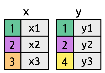
- Let’s define two simple tibbles x and y.
x <- tribble(
  ~key, ~val_x,
     1, "x1",
     2, "x2",
     3, "x3"
)
y <- tribble(
  ~key, ~val_y,
     1, "y1",
     2, "y2",
     4, "y3"
)
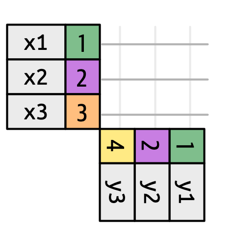
To understand how joins work, it’s useful to think of every possible match.
Here we show that with a grid of connecting lines
3.1 Inner join
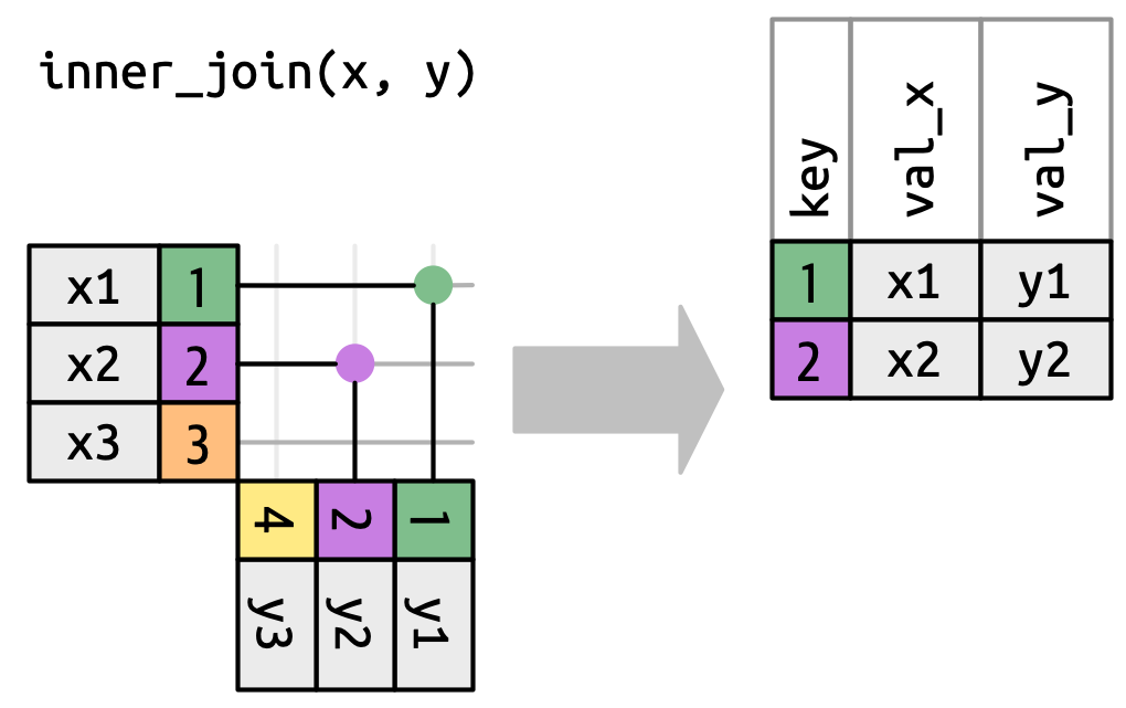
xy <- inner_join(x = x, y = y, by = "key")xy
#> # A tibble: 2 × 3
#> key val_x val_y
#> <dbl> <chr> <chr>
#> 1 1 x1 y1
#> 2 2 x2 y23.2 Left join
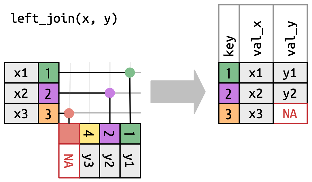
xy_left <- left_join(x = x, y = y, by = "key")xy_left
#> # A tibble: 3 × 3
#> key val_x val_y
#> <dbl> <chr> <chr>
#> 1 1 x1 y1
#> 2 2 x2 y2
#> 3 3 x3 <NA>3.3 Right join
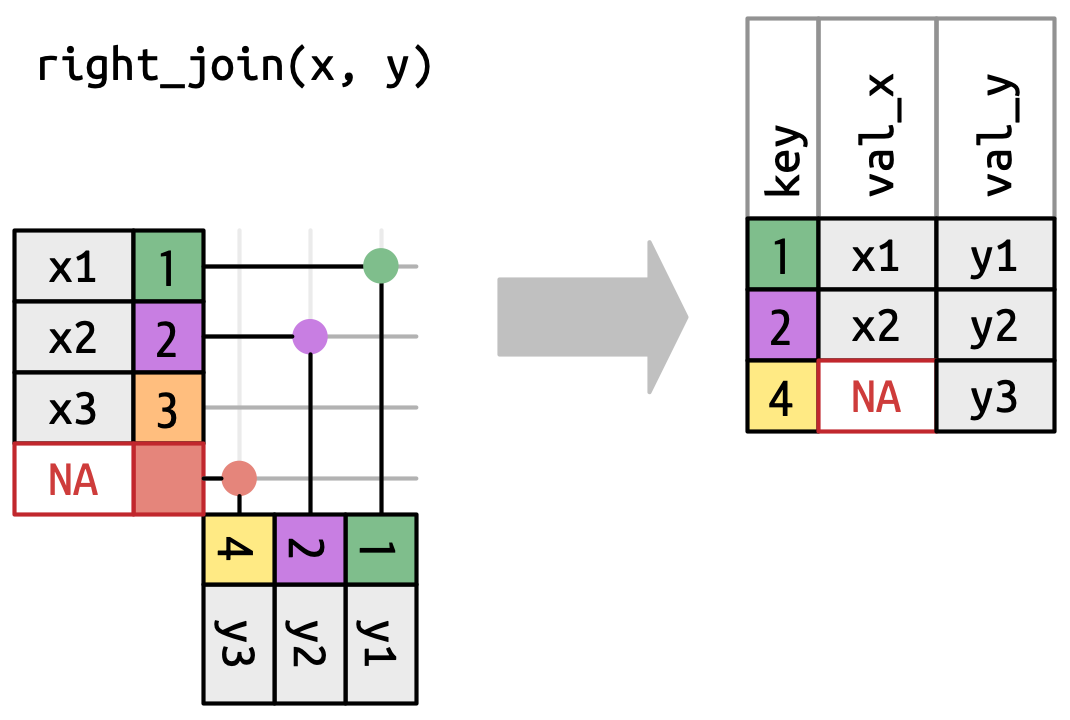
xy_right <- right_join(x = x, y = y,
                    by = "key")
xy_right
#> # A tibble: 3 × 3
#> key val_x val_y
#> <dbl> <chr> <chr>
#> 1 1 x1 y1
#> 2 2 x2 y2
#> 3 4 <NA> y33.4 Full join
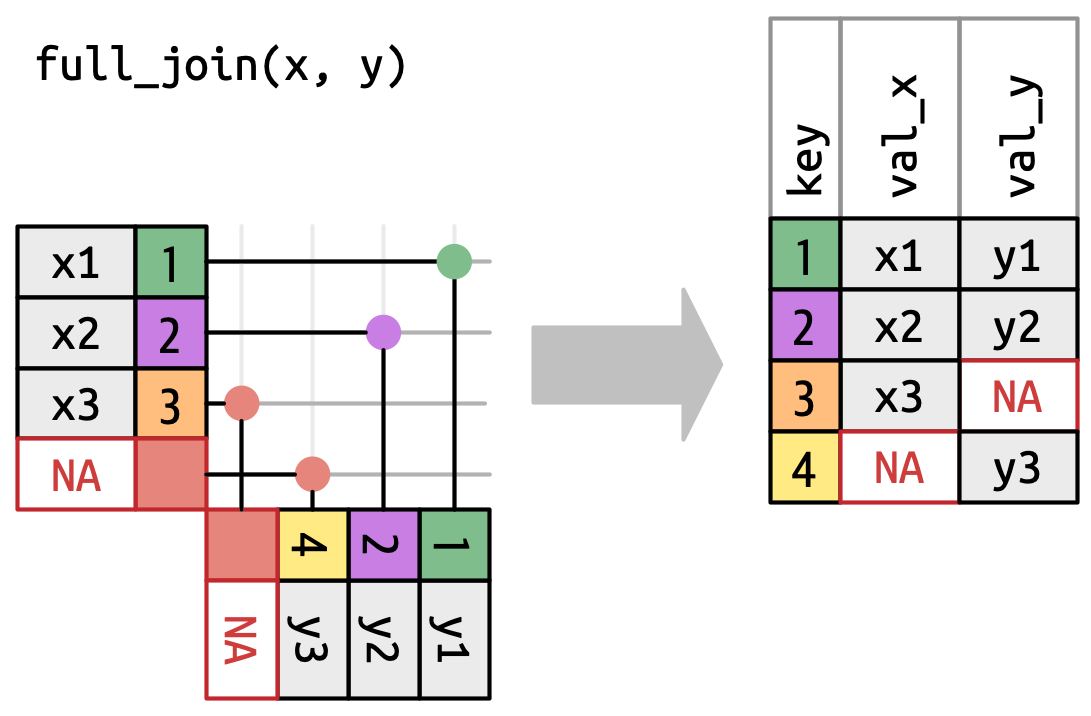
xy_full <- full_join(x = x, y = y, by = "key")xy_full
#> # A tibble: 4 × 3
#> key val_x val_y
#> <dbl> <chr> <chr>
#> 1 1 x1 y1
#> 2 2 x2 y2
#> 3 3 x3 <NA>
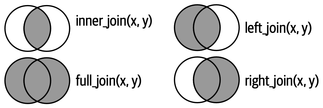
#> 4 4 <NA> y3The following Venn diagrams showing the difference between inner, left, right, and full joins.
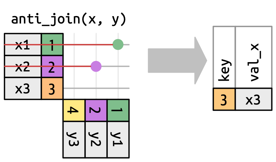
4 Filtering joins
Mutating joins add columns from y to x, matching rows based on the key.
Filtering joins filter rows from \(x\) based on the presence or absence of matches in \(y\).
-
Two types of filtering join:
-
semi_join(), andanti_join()
-
-
semi_join()return all rows from x with a match in y

-
anti_join()keeps rows in x that match zero rows in y
5 Exam data
Year 1
| id | gender | ast101 | ast102 |
|---|---|---|---|
| 101 | F | 57 | 49 |
| 102 | M | 51 | 51 |
| 103 | F | 72 | 26 |
| 104 | F | 58 | 58 |
| 105 | M | 65 | 32 |
| 106 | M | 57 | 62 |
| 107 | F | 65 | 66 |
Year 2
| id | ast201 | ast202 |
|---|---|---|
| 101 | 77 | 43 |
| 102 | 72 | 34 |
| 103 | 65 | 41 |
| 104 | 76 | 39 |
| 105 | 75 | 37 |
| 106 | 70 | 35 |
| 201 | 76 | 65 |
Calculate CGPA, i.e., overall performance of each student
Compare the performance of male and female on the basis of CGPA