10 DS Workflow and Import

1 Data Science Workflow

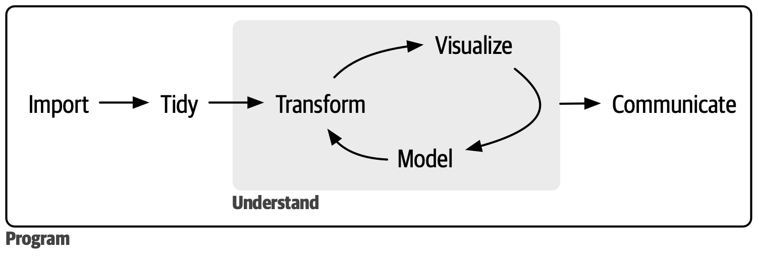
Import

Reading data from different sources, e.g., SAS, SPSS, Stata, Excel, SQL, etc.

Tidy

When your data is tidy, each column is a variable and each row is an observation.

Transform

Transformation includes:
- narrowing in on observations of interest,
- creating new variables that are functions of existing ones,
- calculating summary statistics (counts, means, etc.).

Together, tidying and transforming are called wrangling.

Visualize

Visualization helps you see things you did not expect and raises new questions about your data.

Model

Models summarize data and help answer precise questions.

Communicate

Presenting results and writing reports.

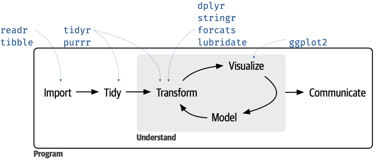
2 The tidyverse

tidyverse is a collection of R packages:
- ggplot2, tibble, tidyr, readr, purrr, dplyr, and many more.
Shared philosophy and consistent design principles.
Code style is different from base R.
Hadley Wickham and colleagues develop tidyverse packages at RStudio Inc.
See: Wickham & Grolemund (2017). R for Data Science.

library(tidyverse)

Loading tidyverse automatically loads ggplot2.

3 Importing Data

Importing data means loading data from external files into R for analysis. Real-world data usually comes from spreadsheets, statistical software, or databases.

library(tidyverse)

Common Data Formats

CSV (.csv)
Excel (.xlsx, .xls)
Text files (.txt)
SPSS (.sav)
Stata (.dta)
SAS (.sas7bdat)
R’s native data (.RData)

Download this data folder for practice.

Importing CSV Files

Using read.csv():

data1 <- read.csv("data/prawnGR.csv")
head(data1)

#>     GRate    diet
#> 1  9.7741 Natural
#> 2 10.2931 Natural
#> 3 10.0474 Natural
#> 4 10.0808 Natural
#> 5  9.3106 Natural
#> 6 10.4414 Natural

Using readr::read_csv():

library(readr)
data1 <- read_csv("data/prawnGR.csv")
head(data1)

#> # A tibble: 6 × 2
#>   GRate diet   
#>   <dbl> <chr>  
#> 1  9.77 Natural
#> 2 10.3  Natural
#> 3 10.0  Natural
#> 4 10.1  Natural
#> 5  9.31 Natural
#> 6 10.4  Natural

Importing Excel Files

Install:

install.packages("readxl")

Read:

library(readxl)
data2 <- read_excel("data/whaledata.xls")
head(data2)

#> # A tibble: 6 × 8
#>   month time.at.station water.noise number.whales latitude longitude depth
#>   <chr>           <dbl> <chr>       <chr>            <dbl>     <dbl> <dbl>
#> 1 May              1344 low         7                 60.4     -4.18   520
#> 2 May              1633 medium      13                60.4     -4.19   559
#> 3 May               743 medium      12                60.5     -4.62  1006
#> 4 May              1050 medium      10                60.3     -4.35   540
#> 5 May              1764 medium      12                60.4     -5.2   1000
#> 6 May               580 high        10                60.4     -5.22  1000
#> # ℹ 1 more variable: gradient <dbl>

Importing Text Files

Using read.table():

data3 <- read.table("data/atmosphere.txt", header = TRUE)
head(data3)

#>   moisture treatment
#> 1    300.6    seeded
#> 2    302.4    seeded
#> 3    298.6    seeded
#> 4    315.9    seeded
#> 5    306.9    seeded
#> 6    300.1    seeded

Importing SPSS Files

Install:

install.packages("haven")

Read:

library(haven)
data4 <- read_sav("data/hw_dat.sav")
head(data4)

#> # A tibble: 6 × 13
#>   year_birth   age division residence religion edu      wealth_index total_birth
#>        <dbl> <dbl> <chr>    <chr>     <chr>    <chr>    <chr>              <dbl>
#> 1       1988    26 Barisal  Rural     Islam    Primary  Poorest                2
#> 2       1973    41 Barisal  Rural     Islam    Primary  Middle                 4
#> 3       1976    38 Barisal  Rural     Islam    Primary  Poorest                2
#> 4       1996    18 Barisal  Rural     Islam    Seconda… Poorest                0
#> 5       1986    28 Barisal  Rural     Islam    Primary  Poorest                2
#> 6       1980    34 Barisal  Rural     Islam    Primary  Poorer                 3
#> # ℹ 5 more variables: current_pregnant <chr>, current_breast_feed <chr>,
#> #   edu_husband <chr>, bmi <dbl>, overweight <dbl>

Importing Stata Files

data5 <- haven::read_dta("data/hw_dat.dta")
head(data5)

#> # A tibble: 6 × 13
#>   year_birth   age division residence religion edu      wealth_index total_birth
#>        <dbl> <dbl> <chr>    <chr>     <chr>    <chr>    <chr>              <dbl>
#> 1       1988    26 Barisal  Rural     Islam    Primary  Poorest                2
#> 2       1973    41 Barisal  Rural     Islam    Primary  Middle                 4
#> 3       1976    38 Barisal  Rural     Islam    Primary  Poorest                2
#> 4       1996    18 Barisal  Rural     Islam    Seconda… Poorest                0
#> 5       1986    28 Barisal  Rural     Islam    Primary  Poorest                2
#> 6       1980    34 Barisal  Rural     Islam    Primary  Poorer                 3
#> # ℹ 5 more variables: current_pregnant <chr>, current_breast_feed <chr>,
#> #   edu_husband <chr>, bmi <dbl>, overweight <dbl>

Importing SAS Files

data6 <- haven::read_sas("data/airline.sas7bdat")
head(data6)

#> # A tibble: 6 × 6
#>    YEAR     Y     W     R     L     K
#>   <dbl> <dbl> <dbl> <dbl> <dbl> <dbl>
#> 1  1948  1.21 0.243 0.145  1.41 0.612
#> 2  1949  1.35 0.260 0.218  1.38 0.559
#> 3  1950  1.57 0.278 0.316  1.39 0.573
#> 4  1951  1.95 0.297 0.394  1.55 0.564
#> 5  1952  2.27 0.310 0.356  1.80 0.574
#> 6  1953  2.73 0.322 0.359  1.93 0.711

Importing R’s native format

load("data/TemoraBR.RData")
head(TemoraBR)

#> # A tibble: 6 × 3
#>    temp beat_rate acclimitisation_temp
#>   <dbl>     <dbl>                <dbl>
#> 1     5      3.76                    5
#> 2     6      5.4                     5
#> 3     7      8                       5
#> 4    10      9.4                     5
#> 5    11     16.6                     5
#> 6    12     18.5                     5

Data Entry in R

Sometimes you need to directly create a tibble:

tibble(
  x = c(1, 2, 5),
  y = c("h", "m", "g"),
  z = c(0.08, 0.83, 0.60)
)

#> # A tibble: 3 × 3
#>       x y         z
#>   <dbl> <chr> <dbl>
#> 1     1 h      0.08
#> 2     2 m      0.83
#> 3     5 g      0.6

Using Built-in Datasets

List datasets:

data()

Load a dataset:

data(mtcars)
head(mtcars)

#>                    mpg cyl disp  hp drat    wt  qsec vs am gear carb
#> Mazda RX4         21.0   6  160 110 3.90 2.620 16.46  0  1    4    4
#> Mazda RX4 Wag     21.0   6  160 110 3.90 2.875 17.02  0  1    4    4
#> Datsun 710        22.8   4  108  93 3.85 2.320 18.61  1  1    4    1
#> Hornet 4 Drive    21.4   6  258 110 3.08 3.215 19.44  1  0    3    1
#> Hornet Sportabout 18.7   8  360 175 3.15 3.440 17.02  0  0    3    2
#> Valiant           18.1   6  225 105 2.76 3.460 20.22  1  0    3    1

Importing Datasets from Packages

Example: gapminder

install.packages("gapminder")

library(gapminder)
data(gapminder)
head(gapminder)

#> # A tibble: 6 × 6
#>   country     continent  year lifeExp      pop gdpPercap
#>   <fct>       <fct>     <int>   <dbl>    <int>     <dbl>
#> 1 Afghanistan Asia       1952    28.8  8425333      779.
#> 2 Afghanistan Asia       1957    30.3  9240934      821.
#> 3 Afghanistan Asia       1962    32.0 10267083      853.
#> 4 Afghanistan Asia       1967    34.0 11537966      836.
#> 5 Afghanistan Asia       1972    36.1 13079460      740.
#> 6 Afghanistan Asia       1977    38.4 14880372      786.

Summary of Importing Functions

CSV, Excel, Text: readr::read_csv(), readxl::read_excel(), read.table()
SPSS, Stata, SAS: haven::read_sav(), haven::read_dta(), haven::read_sas()
RData: load()
R’s built-in data: data()
Data from any R Package: Install the package, use data()

Exporting Data

Exporting to R objects (.RData)

save(mtcars, TemoraBR, file = "two_data_sets.RData")

Exporting to CSV

write.csv(mtcars, "data/mtcars3.csv")
readr::write_excel_csv(mtcars, "data/mtcars4.csv")

Exporting to Text Files

# Export as space-separated text
write.table(mtcars, "mtcars.txt")

# Export as tab-separated text
write.table(mtcars, "mtcars_tab.txt", sep = "\t")

# Export as CSV using write.table
write.table(mtcars, "mtcars_custom.csv",
            sep = ",", row.names = FALSE)