17 {purrr}

Note

This lecture used materials from the iteration chapter in R for data science.

The map functions

The pattern of looping over a vector, doing something to each element and saving the results is so common that the purrr package provides a family of functions to do it for you. There is one function for each type of output:

map() makes a list.
map_lgl() makes a logical vector.
map_int() makes an integer vector.
map_dbl() makes a double vector.
map_chr() makes a character vector.

Each function takes a vector as input, applies a function to each piece, and then returns a new vector that’s the same length (and has the same names) as the input. The type of the vector is determined by the suffix to the map function.

library(purrr) # library(tidyverse) would also work

Imagine we have this simple tibble:

df <- tibble(
  a = rnorm(10),
  b = rnorm(10),
  c = rnorm(10),
  d = rnorm(10)
)

We want to compute the mean, median, and SD of each column

map_dbl(df, mean)

##           a           b           c           d 
## -0.50627203 -0.42086929 -0.40903136  0.08975649

map_dbl(df, median)

##          a          b          c          d 
## -0.2855340 -0.5648310 -0.3025734 -0.2135869

map_dbl(df, sd)

##         a         b         c         d 
## 0.6171634 0.7422437 1.0691040 0.9295846

Compared to using a for loop, focus is on the operation being performed (i.e. mean(), median(), sd()), not the bookkeeping required to loop over every element and store the output. This is even more apparent if we use the pipe:

df |> map_dbl(mean)

##           a           b           c           d 
## -0.50627203 -0.42086929 -0.40903136  0.08975649

df |> map_dbl(median)

##          a          b          c          d 
## -0.2855340 -0.5648310 -0.3025734 -0.2135869

df |> map_dbl(sd)

##         a         b         c         d 
## 0.6171634 0.7422437 1.0691040 0.9295846

The second argument, .f, the function to apply, can be a formula, a character vector, or an integer vector.
map_*() uses $\dots$ ([dot dot dot]) to pass along additional arguments to .f each time it’s called

map_dbl(df, mean, trim = 0.5)

##          a          b          c          d 
## -0.2855340 -0.5648310 -0.3025734 -0.2135869

Look, the map functions also preserve names.

Shortcuts

There are a few shortcuts that you can use with .f in order to save a little typing. Imagine you want to fit a linear model to each group in a dataset. The following toy example splits up the mtcars dataset into three pieces (one for each value of cylinder) and fits the same linear model to each piece:

models <- mtcars |> 
  split(mtcars$cyl) |> 
  map(function(dat) lm(mpg ~ wt, data = dat))
models

## $`4`
## 
## Call:
## lm(formula = mpg ~ wt, data = dat)
## 
## Coefficients:
## (Intercept)           wt  
##      39.571       -5.647  
## 
## 
## $`6`
## 
## Call:
## lm(formula = mpg ~ wt, data = dat)
## 
## Coefficients:
## (Intercept)           wt  
##       28.41        -2.78  
## 
## 
## $`8`
## 
## Call:
## lm(formula = mpg ~ wt, data = dat)
## 
## Coefficients:
## (Intercept)           wt  
##      23.868       -2.192

The syntax for creating an anonymous function in R is quite verbose so purrr provides a convenient shortcut: a one-sided formula

models <- mtcars |>
  split(mtcars$cyl) |>
  map(~lm(mpg ~ wt, data = .))

Here we have used . as a pronoun: it refers to the current list element (in the same way that [i] referred to the current index in the for loop).

When you’re looking at many models, you might want to extract a summary statistic like the $R^{2}$ . To do that we need to first run summary() and then extract the component called r.squared. We could do that using the shorthand for anonymous functions:

models |>
  map(summary) |> 
  map_dbl(~.$r.squared)

##         4         6         8 
## 0.5086326 0.4645102 0.4229655

models |> 
  map(summary) |> 
  map_dbl("r.squared")

##         4         6         8 
## 0.5086326 0.4645102 0.4229655

You can also use an integer to select elements by position:

x <- list(list(1, 2, 3), list(4, 5, 6), list(7, 8, 9))
x |> map_dbl(2)

## [1] 2 5 8

Mapping over multiple arguments

So far we’ve mapped along a single input. But often you have multiple related inputs that you need iterate along in parallel. That’s the job of the map2() and pmap() functions. For example, imagine you want to simulate some random normals with different means and different SDs.

mu <- list(5, 10, -3)
sigma <- list(1, 5, 10)
map2(mu, sigma, rnorm, n = 5) |> str()

## List of 3
##  $ : num [1:5] 5.87 5.19 4.66 6.64 3.68
##  $ : num [1:5] 12.72 6.33 5.68 4.46 17.07
##  $ : num [1:5] 5.29 -11.73 -3.15 1.01 13.79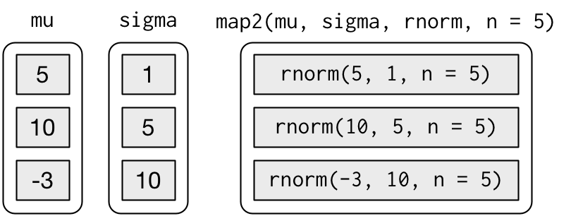

You could also imagine map3(), map4(), map5(), map6() etc, but that would get tedious quickly. Instead, {purrr} provides pmap() which takes a list of arguments

mu <- list(5, 10, -3)
sigma <- list(1, 5, 10)
n <- list(1, 3, 5)
list(n, mu, sigma) |>
  pmap(rnorm) |>
  str()

## List of 3
##  $ : num 5.34
##  $ : num [1:3] 4.72 -2.94 17.51
##  $ : num [1:5] 0.468 0.181 -11.371 2.34 2.545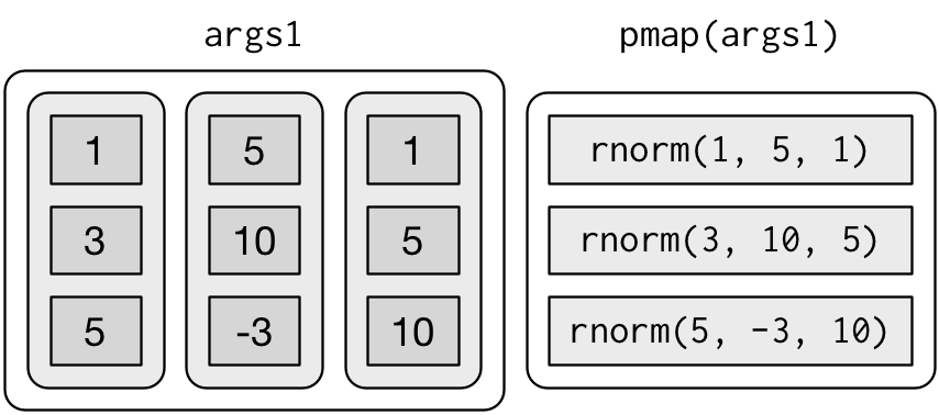

Since the arguments are all the same length, it makes sense to store them in a data frame:

params <- tribble(
  ~mean, ~sd, ~n,
    5,     1,  1,
   10,     5,  3,
   -3,    10,  5
)
params %>% 
  pmap(rnorm)

## [[1]]
## [1] 5.182253
## 
## [[2]]
## [1] 19.639768  1.119090  8.286335
## 
## [[3]]
## [1]  -3.222255  10.904046  16.163897 -12.773508  -6.674612