Probability distributions
1 1 Binomial distribution
Assume \(X\) follows a binomial distribution with parameters \(n\) and \(p\), i.e., \[X\sim B(n, p)\]
Probability mass function \[p(x) = P(X=x) = {n \choose x}p^x (1-p)^{n-x}, x=0, 1, 2, \ldots\]
Cumulative distribution function \[F(x) = P(X\leq x) = \sum_{y = 0}^x P(X=y)\]
- Consider \(B(10, 0.5)\)
dat_binom
#> # A tibble: 11 × 4
#>        x     prob    cprob   cprob1
#>    <int>    <dbl>    <dbl>    <dbl>
#>  1     0 0.000977 0.000977 0.000977
#>  2     1 0.00977  0.0107   0.0107
#>  3     2 0.0439   0.0547   0.0547
#>  4     3 0.117    0.172    0.172
#>  5     4 0.205    0.377    0.377
#>  6     5 0.246    0.623    0.623
#>  7     6 0.205    0.828    0.828
#>  8     7 0.117    0.945    0.945
#>  9     8 0.0439   0.989    0.989
#> 10     9 0.00977  0.999    0.999
#> 11    10 0.000977 1        1
Binomial distribution: PMF
ggplot(data = dat_binom) +
  geom_col(aes(x = x, y = prob))
ggplot(data = dat_binom) +
  geom_col(aes(x = x, y = prob)) +
scale_x_continuous(breaks = 0:10) 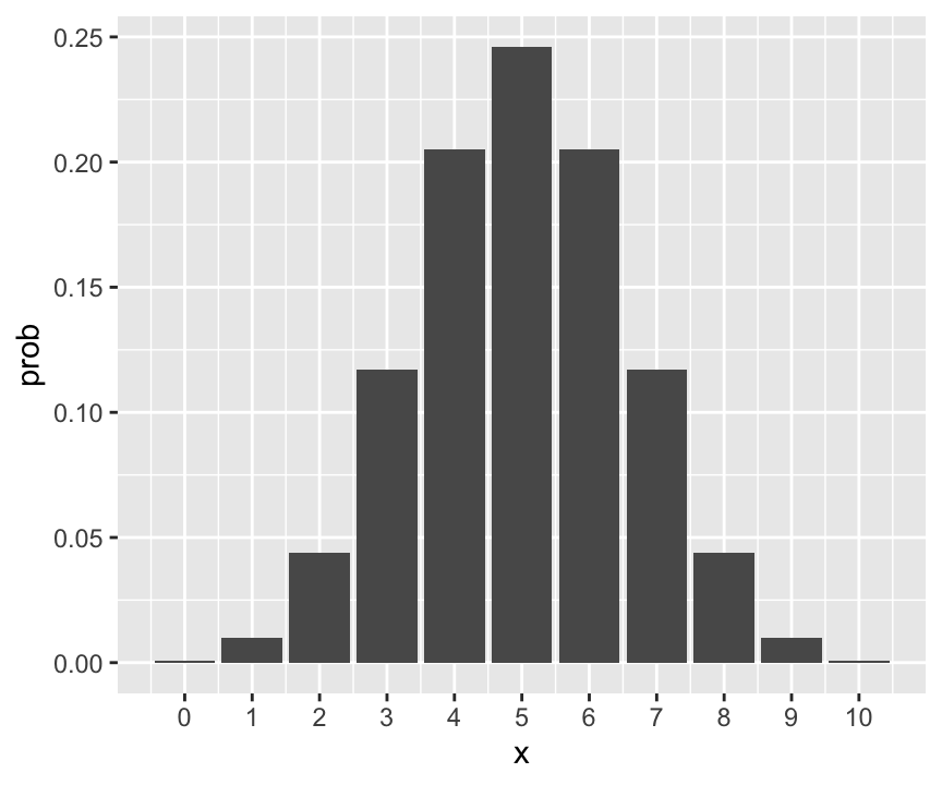
ggplot(data = dat_binom) +
  geom_col(aes(x = x, y = prob), width = .2) +
  scale_x_continuous(breaks = 0:10)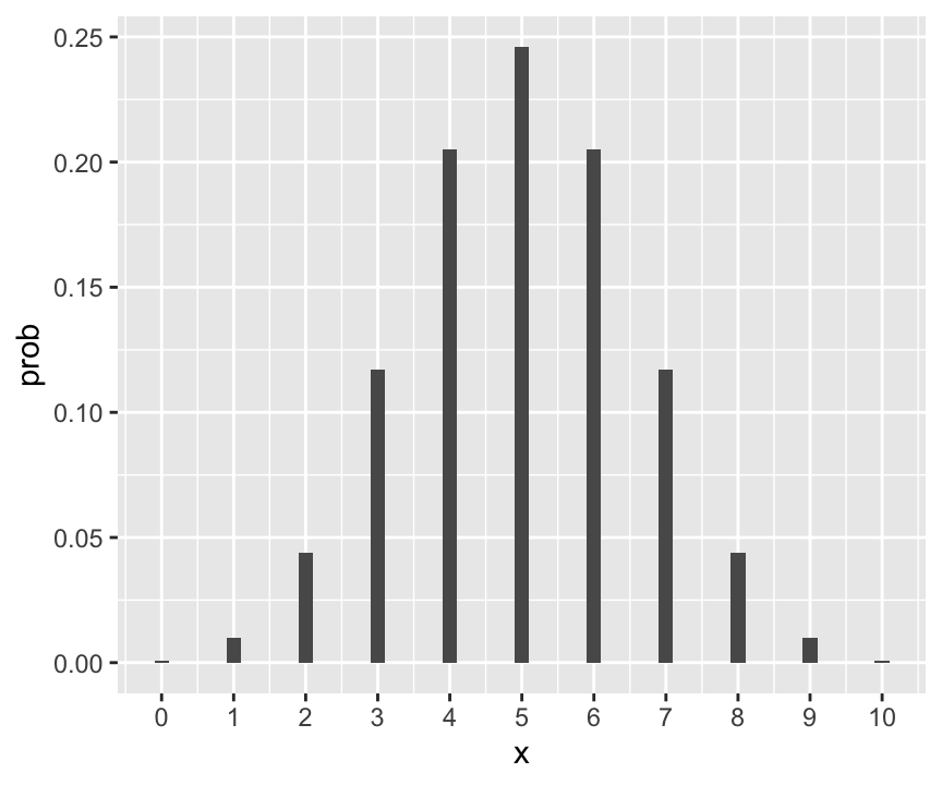
ggplot(data = dat_binom) +
  geom_col(aes(x = x, y = prob), width = .2) +
  scale_x_continuous(breaks = 0:10) +
  theme_minimal(base_size = 18)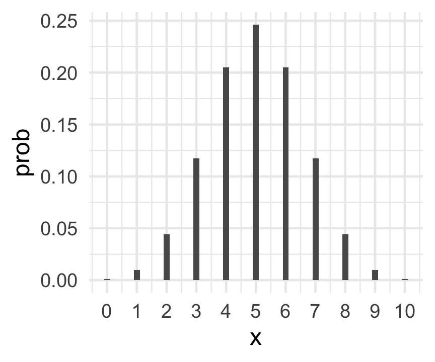
Binomial distribution: CDF
\[F(x) = P(X\leq x) = \sum_{y\leq x} P(X=y)\]
p1 <- ggplot(data = dat_binom) +
  geom_step(aes(x = x, y = cprob)) +
  scale_x_continuous(breaks = 0:10) +
  theme_bw(base_size = 18)
p1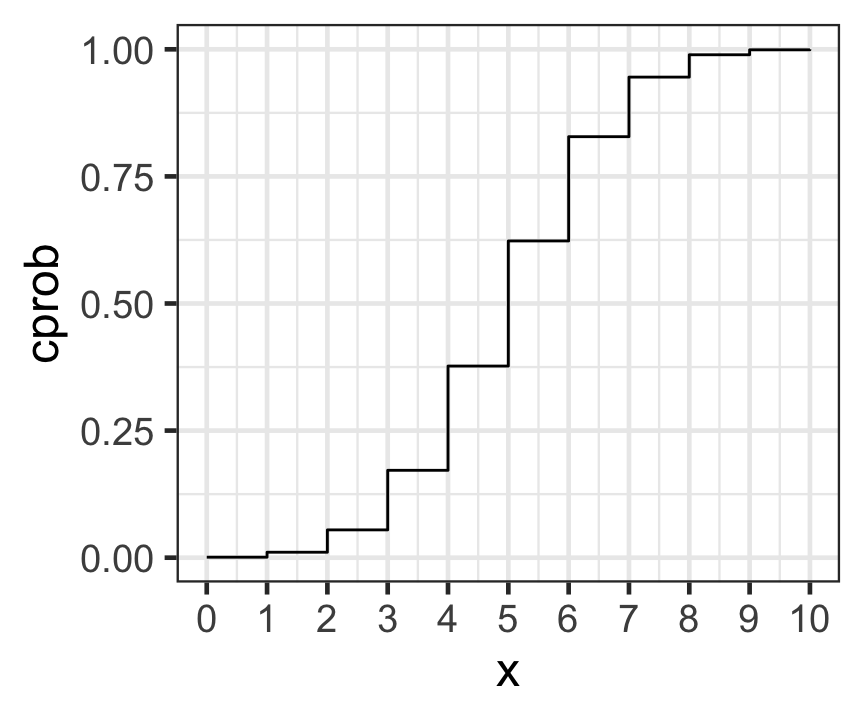
dat1 = tibble(x = dat_binom$x[-1],
              y = dat_binom$cprob[-11])
#
p1 +
  geom_point(aes(x = x, y = cprob), size = 4) +
  geom_point(data = dat1, aes(x = x, y = y),
shape=1, size = 3) 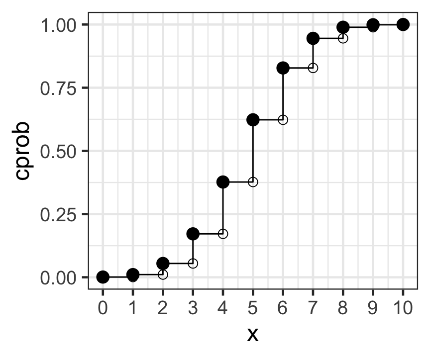
Exercise 3.4.1
-
Plot the probability mass function and cumulative distribution function of binomial distributions:
- \(X\sim B(10, .2)\), (ii) \(X\sim B(10, .90)\)
-
Plot the probability mass function and cumulative distribution function of Poisson distributions:
- \(X\sim Po(.2)\), (ii) \(X\sim Po(5)\)
Show three quartiles (first, second, and third quartile) in the appropriate graphs obtained for earlier questions
2 2 Normal distribution
Assume \(X\) follows a normal distribution, i.e., \(X\sim N(\mu, \sigma^2)\)
-
Probability density function \[f(x) = \frac{1}{\sqrt{2\pi\sigma^2}}e^{-\frac{1}{2}\big(\frac{x-\mu}{\sigma}\big)^2}\]
- \(-\infty <x<\infty\), \(-\infty <\mu<\infty\), and \(\sigma^2>0\)
Standard normal distribution \[Z = \frac{X-\mu}{\sigma}\sim N(0, 1)\]
Cumulative distribution function of standard normal distribution \[\begin{aligned}P(Z\leq z) &= \int_{-\infty}^z \frac{1}{\sqrt{2\pi}}\,e^{-(x^2/2)}dx\\ & = \Phi(z)\end{aligned}\]
dat_norm
#> # A tibble: 1,001 × 3
#>        x        f         F
#>    <dbl>    <dbl>     <dbl>
#>  1 -4    0.000134 0.0000317
#>  2 -3.99 0.000138 0.0000328
#>  3 -3.98 0.000143 0.0000339
#>  4 -3.98 0.000147 0.0000350
#>  5 -3.97 0.000152 0.0000362
#>  6 -3.96 0.000157 0.0000375
#>  7 -3.95 0.000162 0.0000388
#>  8 -3.94 0.000167 0.0000401
#>  9 -3.94 0.000173 0.0000414
#> 10 -3.93 0.000178 0.0000428
#> # ℹ 991 more rows
Normal distribution: PDF
ggplot(dat_norm) +
  geom_line(aes(x, f), size = 2) +
  theme_bw(base_size = 18)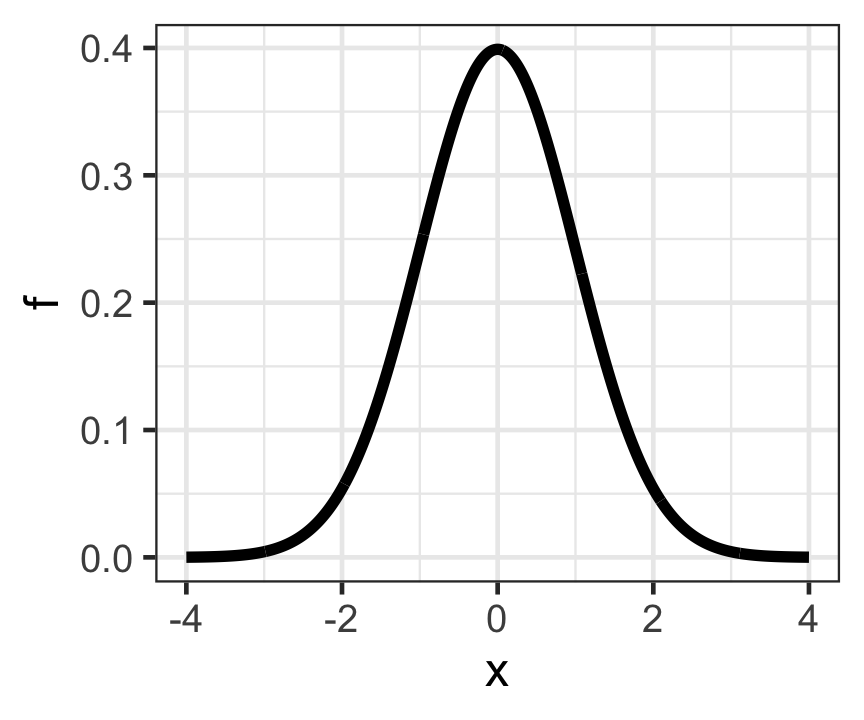
Normal distribution: CDF
ggplot(dat_norm) +
  geom_line(aes(x, F), size = 2) +
  theme_bw(base_size = 18)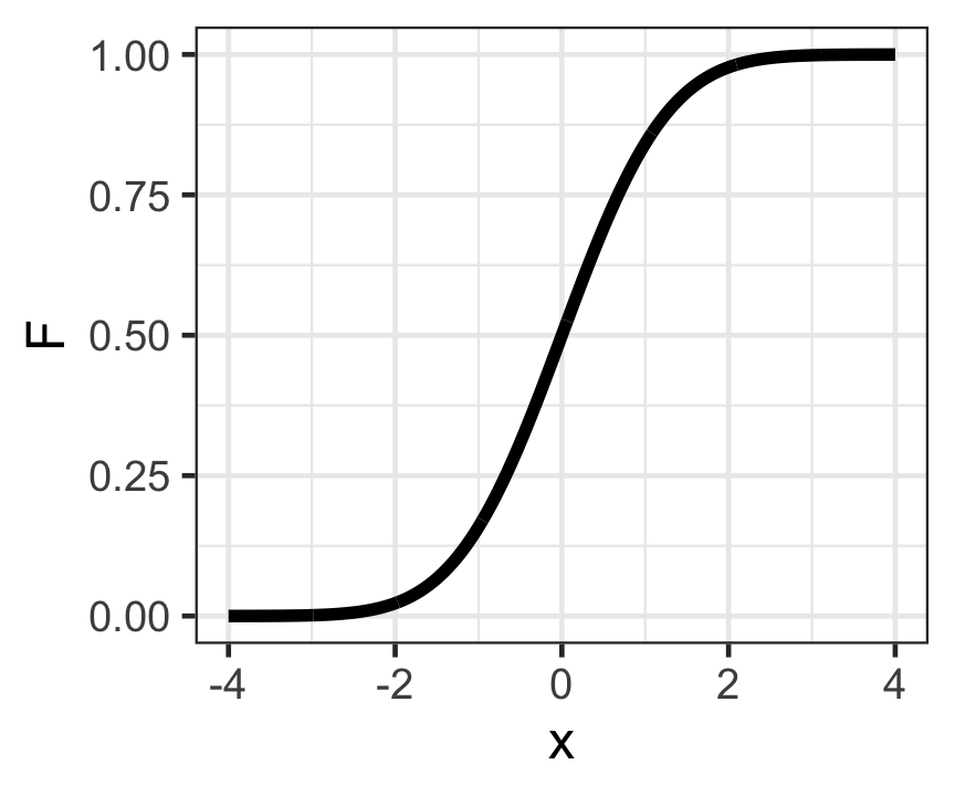
Standard normal distribution: PDF
ggplot(data = tibble(x = c(-4, 4))) +
  stat_function(
    mapping = aes(x = x), fun = dnorm,
    args = list(mean = 0, sd = 1), geom = "line") +
  theme_bw(base_size = 18)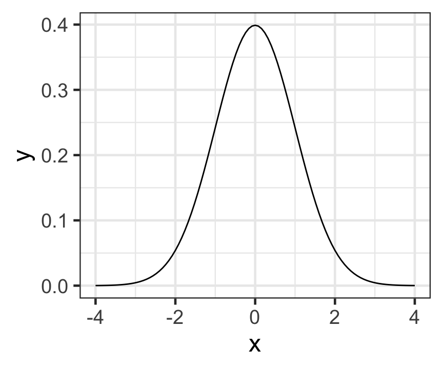
ggplot(data = tibble(x = c(-4, 4))) +
  stat_function(
    mapping = aes(x = x), fun = dnorm,
    geom = "line") +
  stat_function(
    mapping = aes(x = x), fun = dnorm,
    geom = "area", xlim = c(1, 4), fill = "purple") +
  theme_bw(base_size = 18)
- Unspecified
argsargument instat_function()corresponds to standard normal distribution
ggplot(data = tibble(x = c(-4, 4))) +
  stat_function(
    mapping = aes(x = x), fun = dnorm,
    geom = "line") +
  stat_function(
    mapping = aes(x = x), fun = dnorm,
    geom = "area", xlim = c(1, 4), fill = "purple") +
  geom_segment(
    aes(x = 0, xend = 0, y = 0, yend = dnorm(0)),
    col = "blue", size = 1.5) +
  theme_bw(base_size = 18)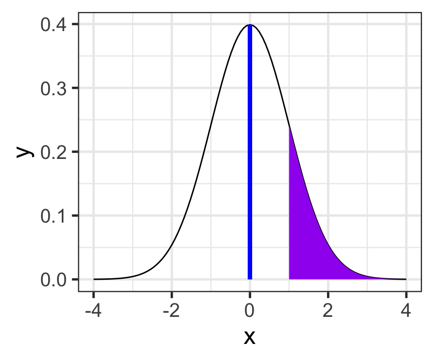
Exercise 3.4.2
Plot density and cumulative distribution functions of \(N(10, 7)\) and \(N(80, 40)\) distributions
Plot density functions of \(N(80, 40)\) and \(N(120, 40)\) distributions on the same plot
Plot density functions of \(N(80, 40)\) and \(N(80, 20)\) distributions on the same plot
Exercise 3..4.3
Plot cumulative distribution functions of \(N(80, 40)\) and \(N(120, 40)\) distributions on the same plot
Plot cumulative distribution functions of \(N(80, 40)\) and \(N(80, 5)\) distributions on the same plot
Plot density and cumulative distribution function of any other distribution that you studies in a course
Summary
Data manipulation and visualizations are briefly discussed at the level so that one can start working with
tidyverse-
The best way to learn R is by reading codes of the experts from their packages and books (
Googleis also helpful)- Knowing the experts for a specific topic is important!
From the beginning, try to use the “best practices” of coding as you write the codes for others (the future yourself is another person!)
Share your knowledge with others as R is free and a product of the volunteer contributions of others!